How an averaged spectrum becomes a map of the Galaxy

Measurement

1. Telescope and SDR measurement

   The dish points at a sky position and the software-defined radio samples a 2.4 MHz-wide band around the hydrogen line. The computer immediately turns short blocks of samples into power spectra with a Fourier transform (1024 frequency channels).

2. Averaged spectrum L0

   A single spectrum is dominated by noise, so thousands are averaged. Every few tens of seconds the software writes one averaged power spectrum to disk. These files are the native data of the project. They are not raw radio samples, and they are on an arbitrary power scale.

3. Metadata and pointing L1

   A scan manifest records the planned sky positions and times. Each averaged spectrum is matched to a position by its timestamp. The manifest stores the commanded position, not an independent measurement of where the dish pointed, which is one reason pointing checks matter.

Reduction

4. Baseline and bandpass L2

   The receiver's response is not flat across the band. A smooth baseline is fitted to line-free channels on either side of the hydrogen line and removed, leaving the line as a small excess over the baseline. For wide native spectra, a bandpass template measured from the session itself removed a strong slope. The result is a relative scale, usually quoted in dB above the baseline.

5. RFI handling

   Radio-frequency interference is anything that is not sky signal. DISH222 sees a permanent spur exactly at 1420.000 MHz and narrow spurs from its motors. Real Galactic hydrogen is broad, so a minimum line width filters out narrow spikes. Quality gates reject spectra whose line-free channels are not flat: in the 26 Aug session 661 of 776 spectra passed.

6. H I line measurement

   After baseline removal the line strength is expressed as a fractional excess over the baseline:

   f = P_line / P_baseline - 1 = 10^(x/10) - 1

   where x is the line height in dB. Two summaries appear in the archive: the peak of a smoothed spectrum (26 Aug products) and the intensity-weighted mean velocity, or first moment (2–3 Sep products). They answer different questions and are not directly comparable.

Physics

7. Frequency to radial velocity

   Gas moving away from us shifts the line to lower frequency. The Doppler formula converts an observed frequency into a velocity relative to the telescope:

   v_topo = c (f0 - f_obs) / f0, f0 = 1420.40575 MHz

   The Earth's rotation and orbit, and the Sun's motion, are then removed so that velocities refer to the Local Standard of Rest (LSR). For the 26 Aug products this meant adding a barycentric correction and the standard 20 km/s solar motion towards RA 18h03m50s, Dec +30°00′17″.

8. Calibration L3

   Calibration turns the relative line strength into a brightness temperature in kelvin. The current reference scale (C4) is

   T_B = (f - p) G

   with a conversion constant G and a small pedestal p. The scale went through five stages, and every archived product keeps the stage it was made with. See Calibration.

9. Sky positioning

   Each spectrum is assigned the sky coordinates of its pointing and converted between equatorial (RA, Dec) and Galactic (l, b) frames. Spectra taken within about one beam radius of each other are stacked to reduce noise. With a beam about 3° wide, every map is inevitably smooth on scales smaller than a few degrees.

Products and interpretation

10. Spectral cube L4

    Gridding spectra onto regular sky pixels, with velocity as the third axis, gives a position–position–velocity cube (FITS format). The 26 Aug cube covers l 146°–228°, b −12° to +22° and −120 to +60 km/s. See the lecture on data cubes.

11. Maps and science products L5 L6

    Collapsing the cube gives maps: peak brightness, velocity (moment maps) and catalogues. Curated products go further, combining sessions or applying selection rules and corrections. Every such step changes what the product can be used for, so it is recorded.

12. Comparison with reference surveys

    The Leiden/Argentine/Bonn (LAB) survey is a professional all-sky H I survey. Comparing DISH222 with LAB smoothed to a 3° beam tests shapes, velocities and brightness. It is a validation, and in C4 also the reference for the kelvin scale, so it is not an independent absolute calibration. Known reasons for differences are beam dilution, stray radiation entering through sidelobes, baseline choices and pointing.

    

13. Interpretation

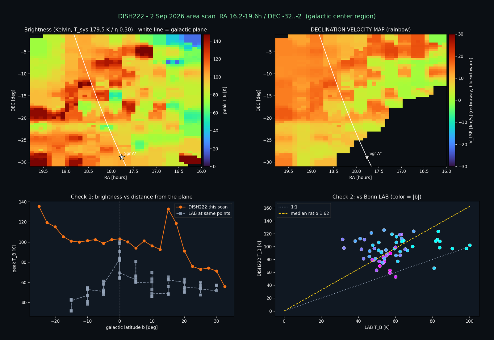
    Velocities along a line of sight map onto distance through the Galaxy's rotation, which is how spiral arms and the rotation curve are traced. Interpretation is the last step for a reason: it inherits every limitation above. In the project's early comparison with LAB (on the relative scale), the velocity–longitude pattern of the outer Galaxy matched LAB closely, but the peak metric compressed the rotation amplitude by roughly a factor of four.