Interactive Lecture

The Story, the System, and the Science

A 52-slide web version of the Radio Telescope / H I 21-cm lecture.

Slide 1 / 52 Back to top
Slide 001 / 052

قصة تطوير التلسكوب الراديوي
Original PowerPoint slide 001: قصة تطوير التلسكوب الراديوي

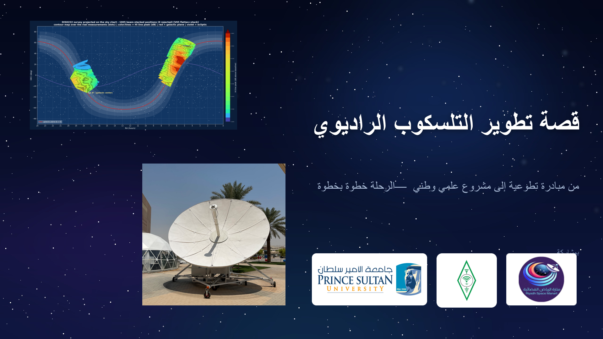
تفتح الشريحة المحاضرة بوصفها قصة تطور مشروع، لا مجرد شرح علمي منفصل. ظهور الجهات المشاركة يضع المشروع في سياقه الوطني والتطوعي، ويُمهّد لتتبع الرحلة من الفكرة إلى منظومة رصد قادرة على إنتاج بيانات فلكية.

تفاصيل أكثر
  • قصة تطوير التلسكوب الراديوي
  • من مبادرة تطوعية إلى مشروع علمي وطني — الرحلة خطوة بخطوة
  • بمشاركة
Slide 002 / 052

تأسيس الجمعية ووضع الاستراتيجية

Original PowerPoint slide 002: تأسيس الجمعية ووضع الاستراتيجية

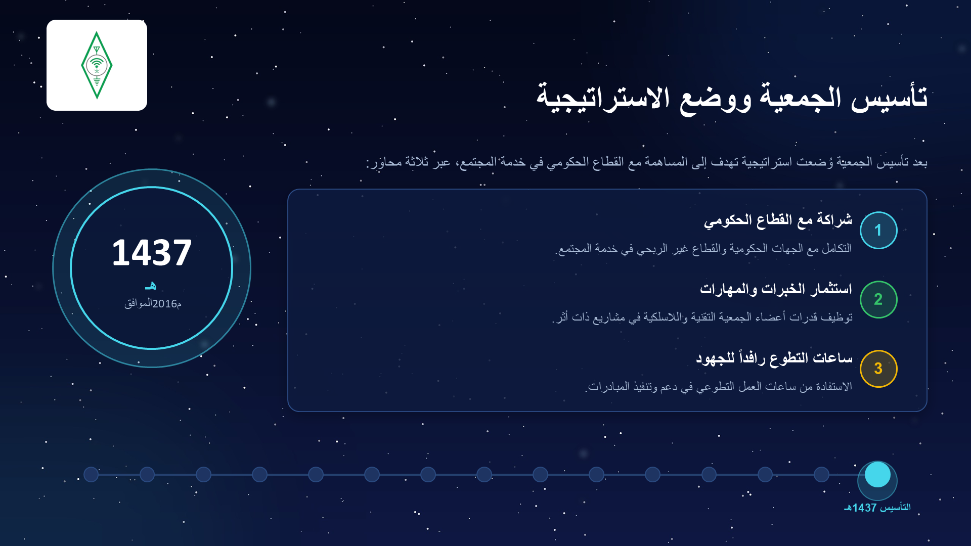
توضح الشريحة نقطة البداية المؤسسية: تأسيس الجمعية عام 1437هـ / 2016م وصياغة استراتيجية لخدمة المجتمع عبر خبرات الأعضاء وساعات التطوع. هذه الخلفية مهمة لأنها تفسر لماذا بدأ المشروع بروح مبادرة محلية قبل أن يتحول إلى عمل هندسي وعلمي أوسع.

تفاصيل أكثر
  • تأسيس الجمعية ووضع الاستراتيجية
  • 1437
  • هـ
  • الموافق 2016م
  • بعد تأسيس الجمعية وُضعت استراتيجية تهدف إلى المساهمة مع القطاع الحكومي في خدمة المجتمع، عبر ثلاثة محاور:
  • 1
  • شراكة مع القطاع الحكومي
  • التكامل مع الجهات الحكومية والقطاع غير الربحي في خدمة المجتمع.
  • 2
  • استثمار الخبرات والمهارات
  • توظيف قدرات أعضاء الجمعية التقنية واللاسلكية في مشاريع ذات أثر.
  • 3
  • ساعات التطوع رافداً للجهود
  • الاستفادة من ساعات العمل التطوعي في دعم وتنفيذ المبادرات.
  • التأسيس 1437هـ
Slide 003 / 052

الاجتماع التأسيسي وانطلاق المشروع

Original PowerPoint slide 003: الاجتماع التأسيسي وانطلاق المشروع

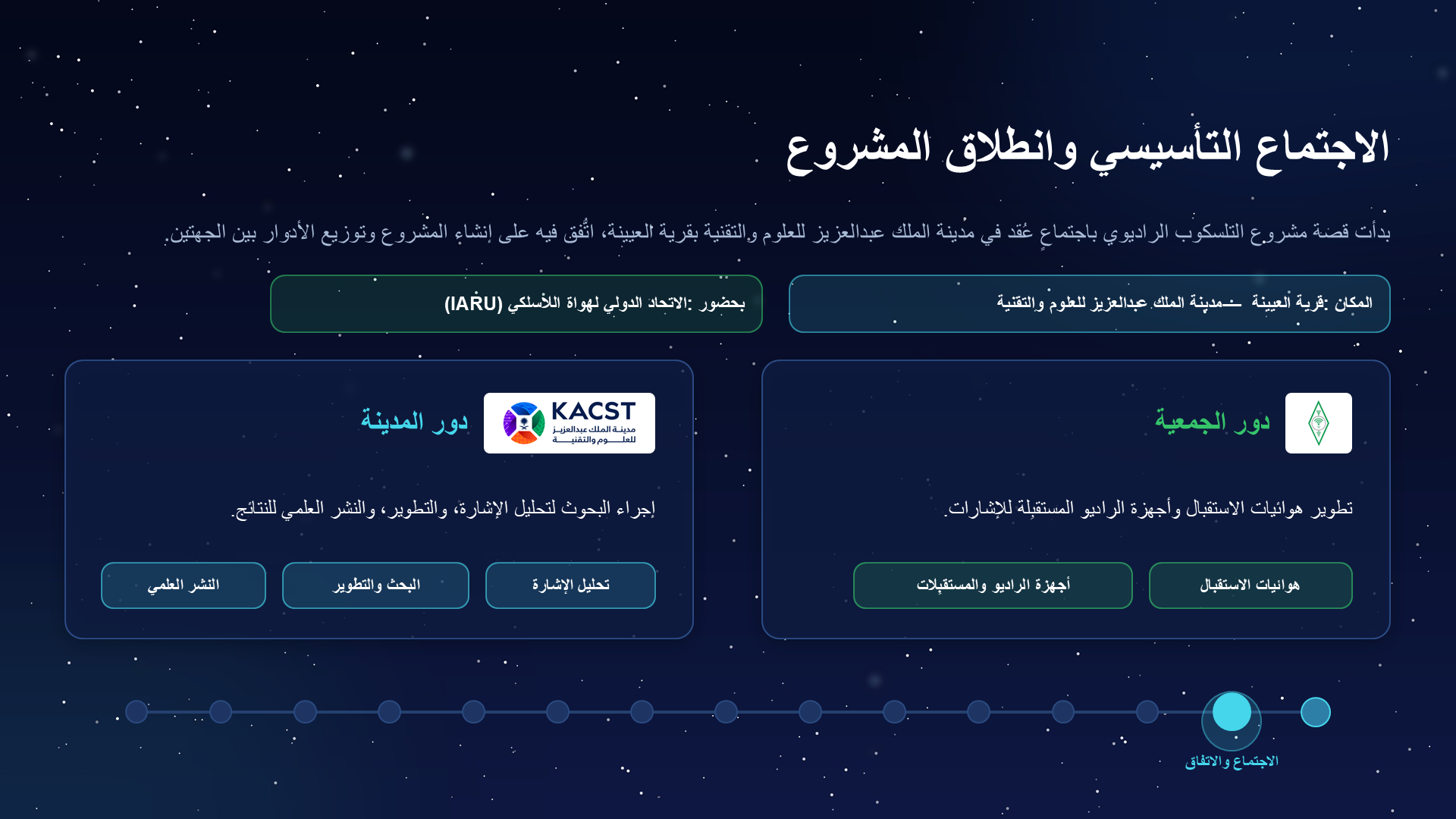
تسجل هذه الشريحة لحظة انطلاق المشروع عملياً من اجتماع مدينة الملك عبدالعزيز للعلوم والتقنية في العيينة. الأهم هنا هو توزيع الأدوار: تطوير الهوائيات وأجهزة الراديو من جهة، والبحث وتحليل الإشارة والتطوير من جهة أخرى، وهو التقسيم الذي سيظهر أثره لاحقاً في تكامل المنظومة.

تفاصيل أكثر
  • الاجتماع التأسيسي وانطلاق المشروع
  • بدأت قصة مشروع التلسكوب الراديوي باجتماعٍ عُقد في مدينة الملك عبدالعزيز للعلوم والتقنية بقرية العيينة، اتُّفق فيه على إنشاء المشروع وتوزيع الأدوار بين الجهتين.
  • المكان: قرية العيينة — مدينة الملك عبدالعزيز للعلوم والتقنية
  • بحضور: الاتحاد الدولي لهواة اللاسلكي (IARU)
  • دور الجمعية
  • تطوير هوائيات الاستقبال وأجهزة الراديو المستقبِلة للإشارات.
  • هوائيات الاستقبال
  • أجهزة الراديو والمستقبِلات
  • دور المدينة
  • إجراء البحوث لتحليل الإشارة، والتطوير، والنشر العلمي للنتائج.
  • تحليل الإشارة
  • البحث والتطوير
  • النشر العلمي
  • الاجتماع والاتفاق
Slide 004 / 052

اجتماعات التنسيق والقرار المفصلي

Original PowerPoint slide 004: اجتماعات التنسيق والقرار المفصلي

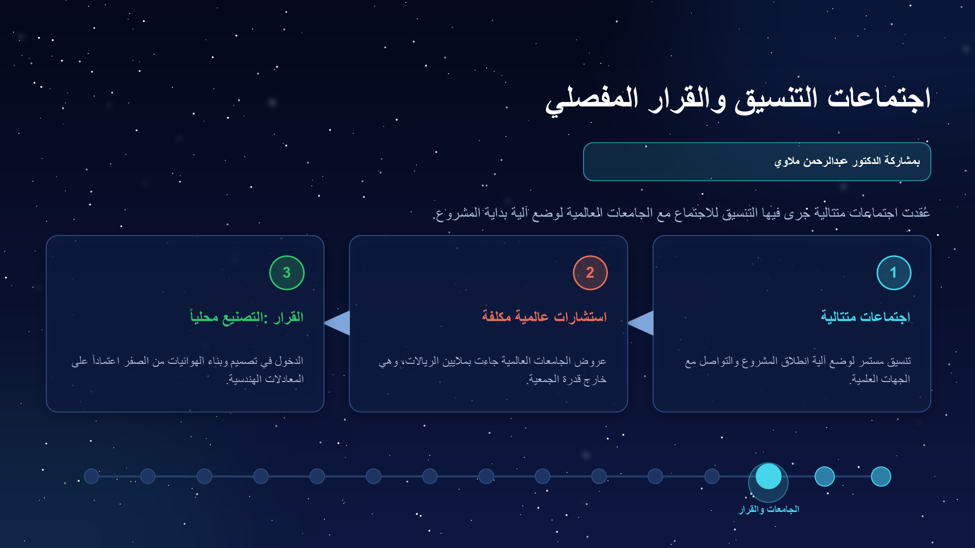
تبيّن الشريحة أن المسار لم يكن شراء حل جاهز، بل قراراً مفصلياً بالتصميم والبناء محلياً بعد أن ظهرت كلفة الاستشارات العالمية خارج قدرة الجمعية. هذه اللحظة حوّلت المشروع إلى تحدٍ هندسي تعليمي قائم على التعلم والتجريب.

تفاصيل أكثر
  • اجتماعات التنسيق والقرار المفصلي
  • بمشاركة الدكتور عبدالرحمن ملاوي
  • عُقدت اجتماعات متتالية جرى فيها التنسيق للاجتماع مع الجامعات العالمية لوضع آلية بداية المشروع.
  • 1
  • اجتماعات متتالية
  • تنسيق مستمر لوضع آلية انطلاق المشروع والتواصل مع الجهات العلمية.
  • 2
  • استشارات عالمية مكلفة
  • عروض الجامعات العالمية جاءت بملايين الريالات، وهي خارج قدرة الجمعية.
  • 3
  • القرار: التصنيع محلياً
  • الدخول في تصميم وبناء الهوائيات من الصفر اعتماداً على المعادلات الهندسية.
  • الجامعات والقرار
Slide 005 / 052

من المعادلات إلى التصميم

Original PowerPoint slide 005: من المعادلات إلى التصميم

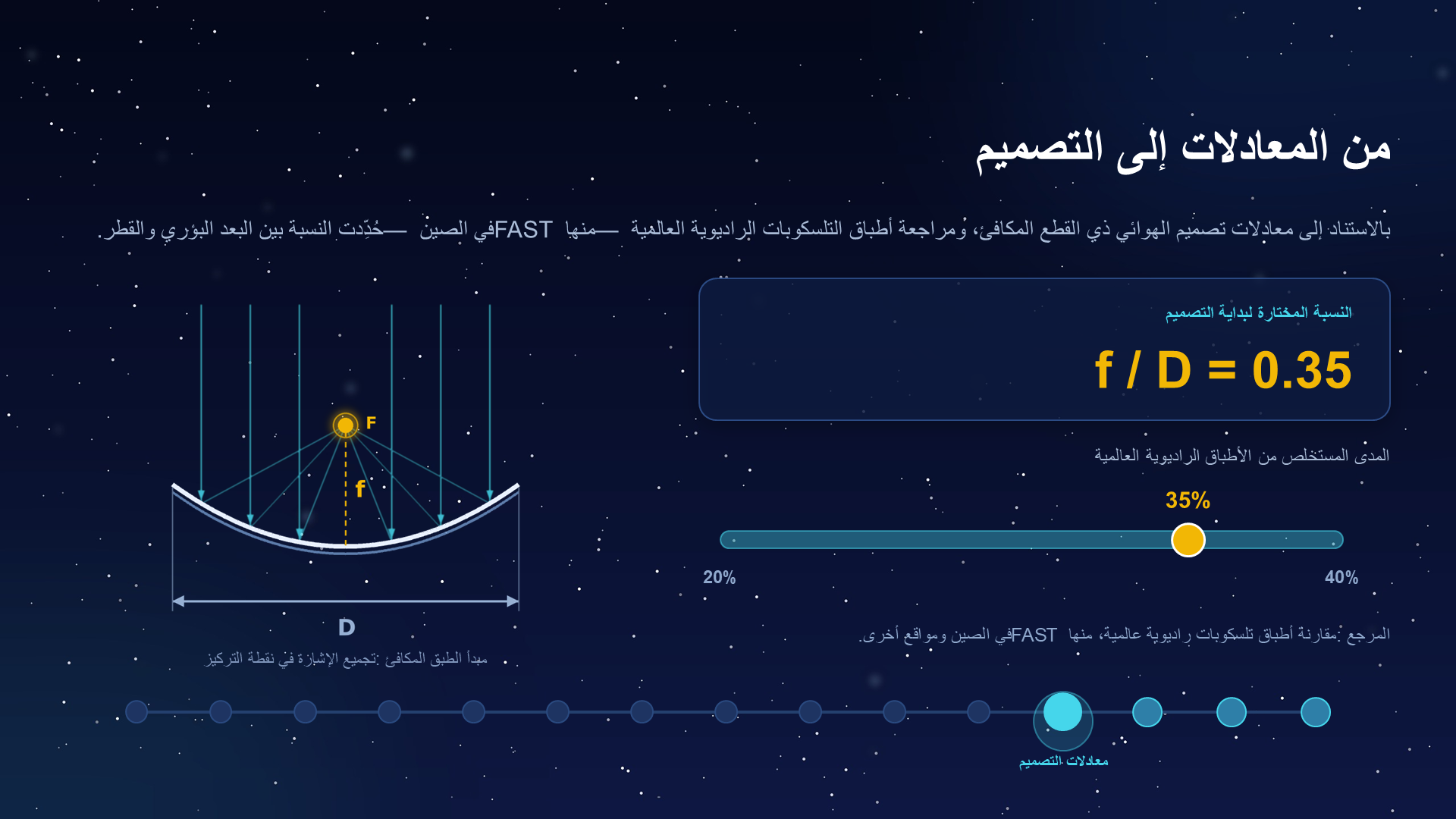
هنا يبدأ التصميم الهندسي الحقيقي للطبق المكافئ. اختيار النسبة \(\frac{f}{D}=0.35\) يعني تحديد علاقة البعد البؤري بقطر الطبق بحيث تُجمع الإشارة الراديوية عند نقطة التركيز. الشريحة تربط بين معادلات التصميم ومقارنة أطباق عالمية مثل FAST، ثم تختار قيمة عملية كبداية للتصنيع المحلي.

تفاصيل أكثر
  • من المعادلات إلى التصميم
  • بالاستناد إلى معادلات تصميم الهوائي ذي القطع المكافئ، ومراجعة أطباق التلسكوبات الراديوية العالمية — منها FAST في الصين — حُدِّدت النسبة بين البعد البؤري والقطر.
  • مبدأ الطبق المكافئ: تجميع الإشارة في نقطة التركيز
  • النسبة المختارة لبداية التصميم
  • f / D = 0.35
  • المدى المستخلص من الأطباق الراديوية العالمية
  • 35%
  • 20%
  • 40%
  • المرجع: مقارنة أطباق تلسكوبات راديوية عالمية، منها FAST في الصين ومواقع أخرى.
  • معادلات التصميم
Slide 006 / 052

الخطوة الخامسة

Original PowerPoint slide 006: الخطوة الخامسة

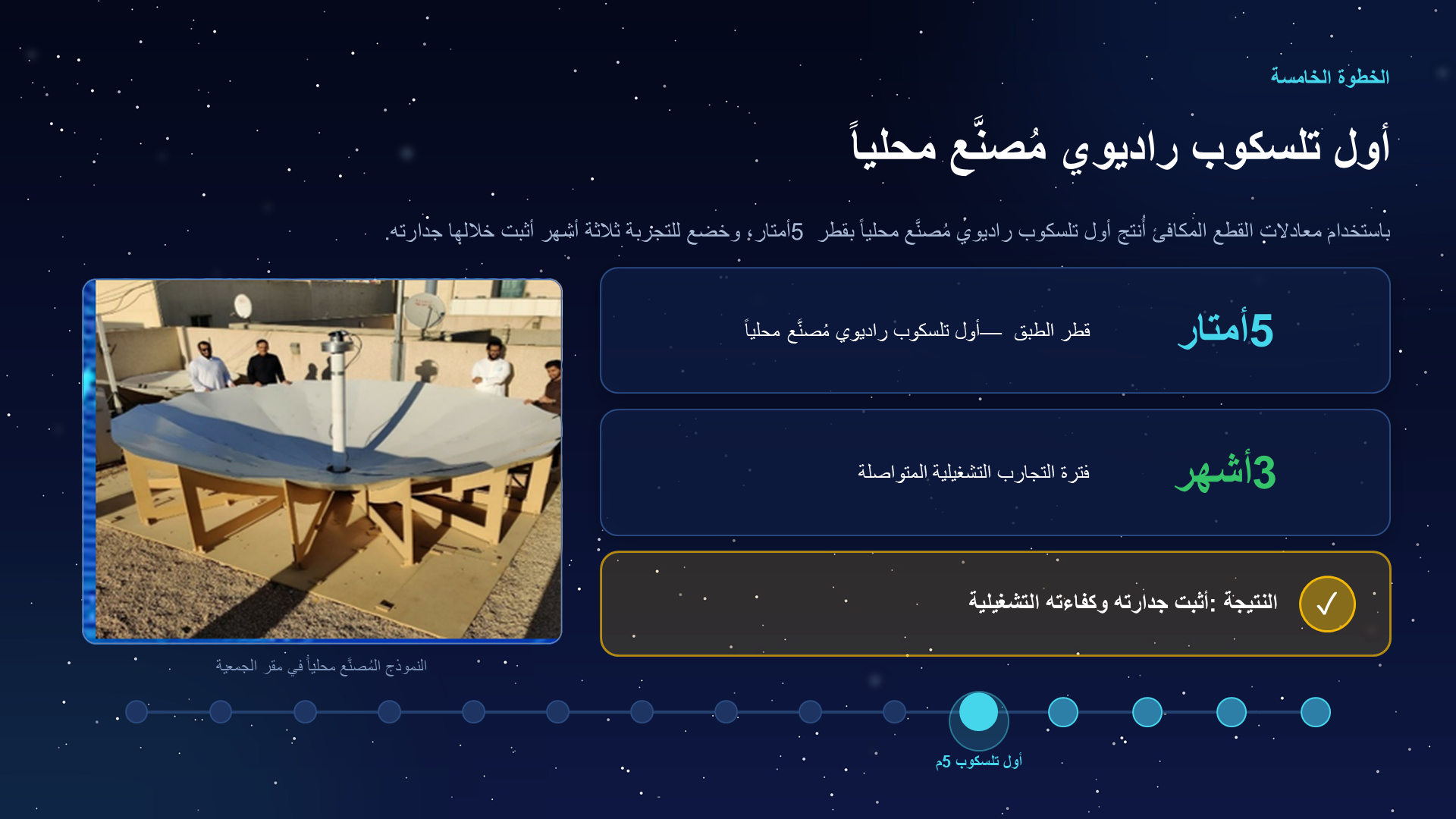
تعرض الشريحة نتيجة التحول من الحساب إلى التصنيع: أول تلسكوب راديوي محلي بقطر 5 أمتار. فترة الاختبار لثلاثة أشهر مهمة لأنها تشير إلى أن النموذج لم يكن شكلياً فقط، بل خضع لتجربة عملية أثبتت جدواه قبل التوسع.

تفاصيل أكثر
  • الخطوة الخامسة
  • أول تلسكوب راديوي مُصنَّع محلياً
  • باستخدام معادلات القطع المكافئ أُنتج أول تلسكوب راديوي مُصنَّع محلياً بقطر 5 أمتار، وخضع للتجربة ثلاثة أشهر أثبت خلالها جدارته.
  • النموذج المُصنَّع محلياً في مقر الجمعية
  • 5 أمتار
  • قطر الطبق — أول تلسكوب راديوي مُصنَّع محلياً
  • 3 أشهر
  • فترة التجارب التشغيلية المتواصلة
  • النتيجة: أثبت جدارته وكفاءته التشغيلية
  • أول تلسكوب 5م
Slide 007 / 052

من نموذج واحد إلى انتشار وطني

Original PowerPoint slide 007: من نموذج واحد إلى انتشار وطني

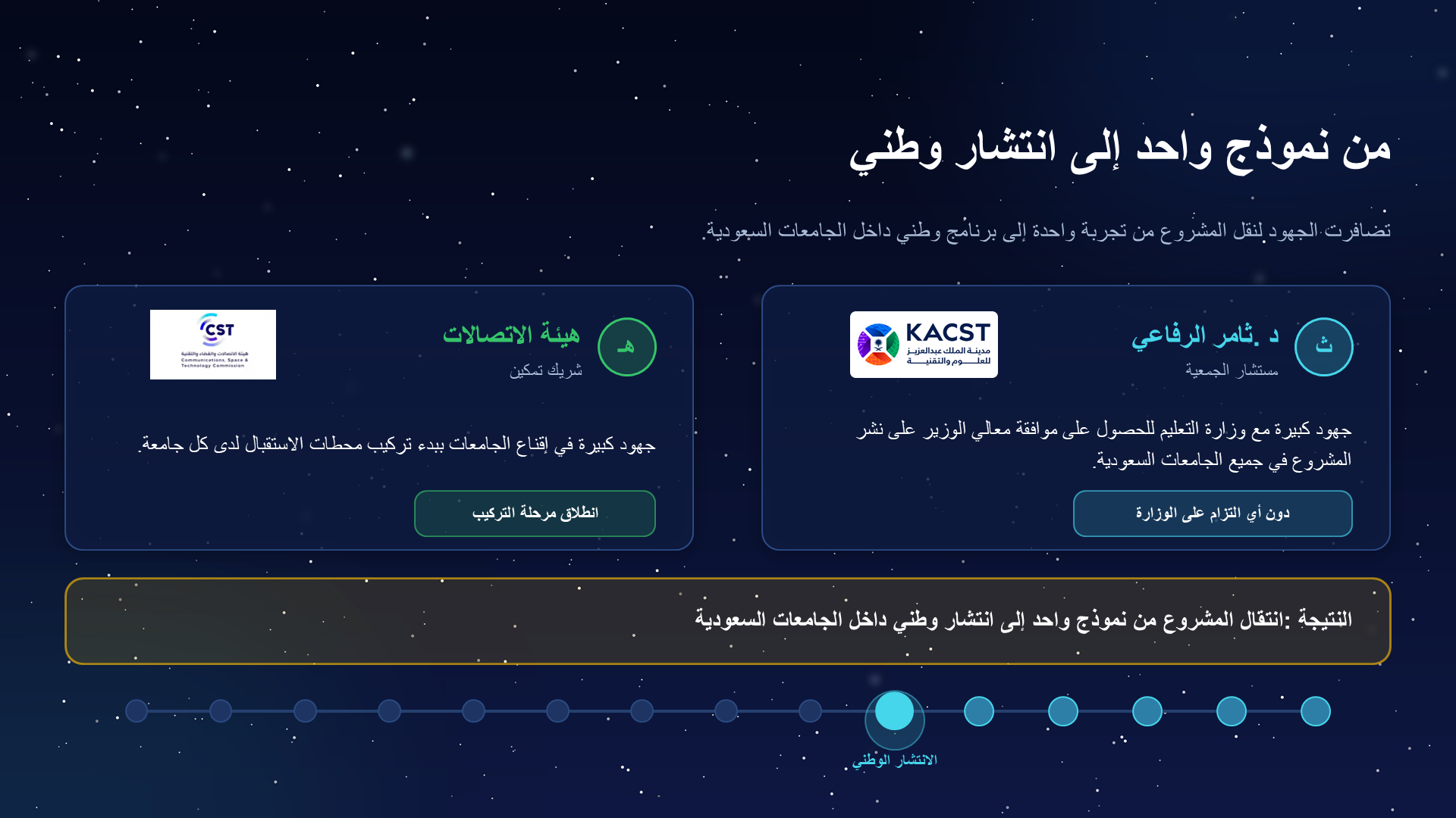
تنتقل الشريحة من نموذج واحد إلى فكرة الانتشار الوطني داخل الجامعات السعودية. دور التواصل المؤسسي هنا أساسي؛ فنجاح التلسكوب الأول فتح باب تحويله إلى برنامج تعليمي وبحثي أوسع بدلاً من بقائه تجربة منفردة.

تفاصيل أكثر
  • من نموذج واحد إلى انتشار وطني
  • تضافرت الجهود لنقل المشروع من تجربة واحدة إلى برنامج وطني داخل الجامعات السعودية.
  • ث
  • د. ثامر الرفاعي
  • مستشار الجمعية
  • جهود كبيرة مع وزارة التعليم للحصول على موافقة معالي الوزير على نشر المشروع في جميع الجامعات السعودية.
  • دون أي التزام على الوزارة
  • هـ
  • هيئة الاتصالات
  • شريك تمكين
  • جهود كبيرة في إقناع الجامعات ببدء تركيب محطات الاستقبال لدى كل جامعة.
  • انطلاق مرحلة التركيب
  • النتيجة: انتقال المشروع من نموذج واحد إلى انتشار وطني داخل الجامعات السعودية
  • الانتشار الوطني
Slide 008 / 052

مواقع تركيب محطات التلسكوب الراديوي

Original PowerPoint slide 008: مواقع تركيب محطات التلسكوب الراديوي

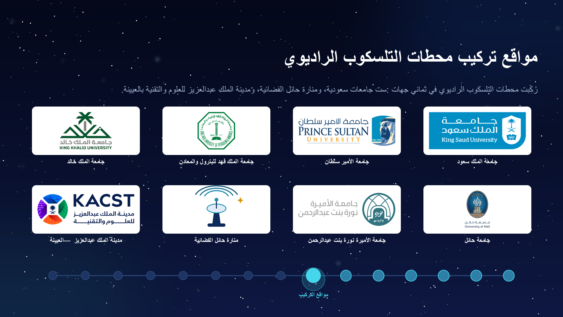
توثق الشريحة مواقع تركيب محطات التلسكوب الراديوي كما يعرضها المصدر: ست جامعات سعودية إضافة إلى منارة حائل الفضائية ومدينة الملك عبدالعزيز للعلوم والتقنية في العيينة. هذه الخريطة الميدانية تجعل المشروع شبكة رصد وتدريب، لا جهازاً واحداً فقط.

تفاصيل أكثر
  • مواقع تركيب محطات التلسكوب الراديوي
  • رُكِّبت محطات التلسكوب الراديوي في ثماني جهات: ست جامعات سعودية، ومنارة حائل الفضائية، ومدينة الملك عبدالعزيز للعلوم والتقنية بالعيينة.
  • جامعة الملك سعود
  • جامعة الأمير سلطان
  • جامعة الملك فهد للبترول والمعادن
  • جامعة الملك خالد
  • جامعة حائل
  • جامعة الأميرة نورة بنت عبدالرحمن
  • منارة حائل الفضائية
  • مدينة الملك عبدالعزيز — العيينة
  • مواقع التركيب
Slide 009 / 052

نماذج المحطات المُركَّبة على أرض الواقع

Original PowerPoint slide 009: نماذج المحطات المُركَّبة على أرض الواقع

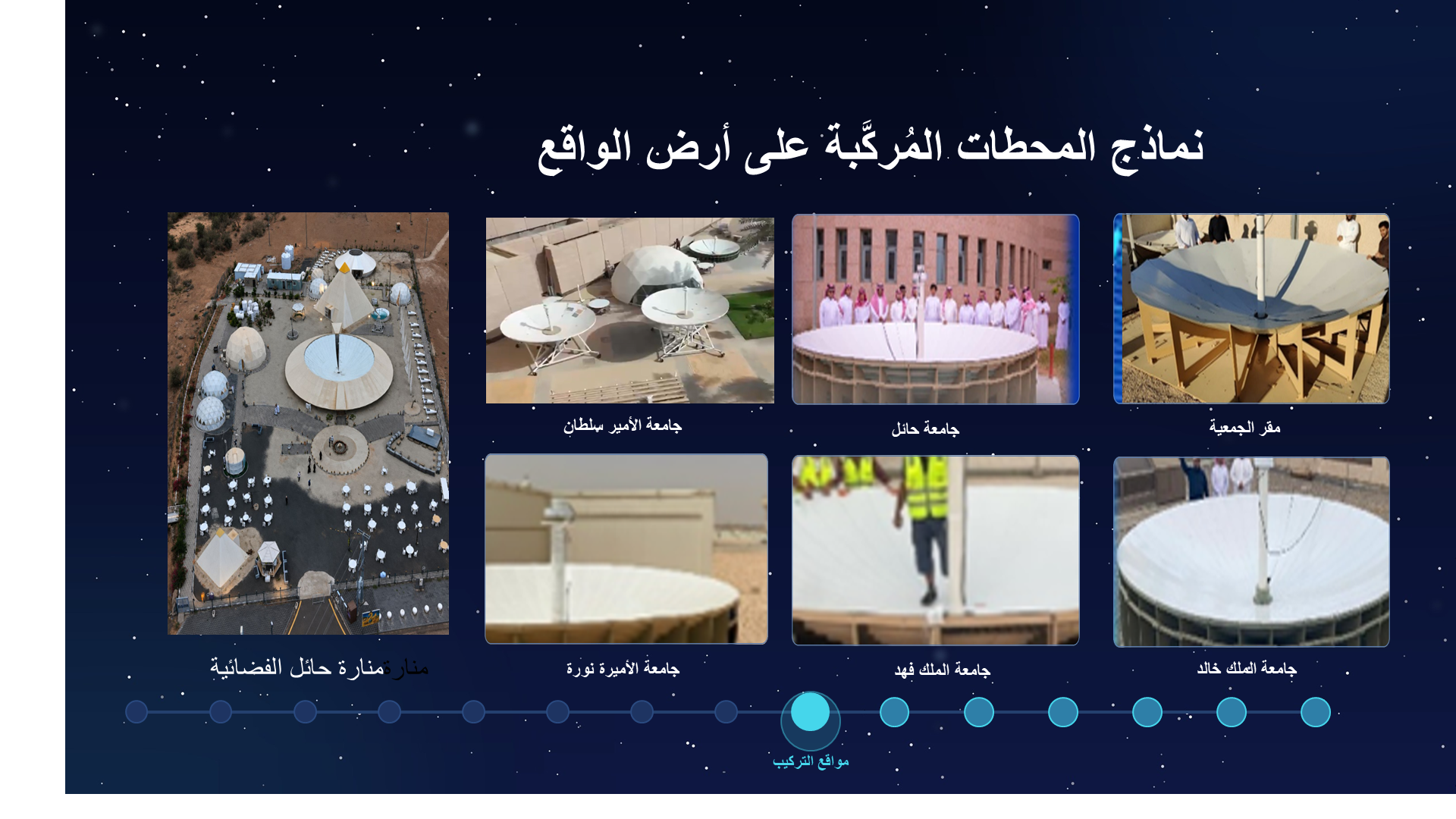
تُظهر الصور أن المحطات لم تبقَ على مستوى المخطط؛ بل وصلت إلى مواقع فعلية مثل مقر الجمعية وجامعة حائل وجامعة الأمير سلطان. قيمة هذه الشريحة أنها تقدم دليلاً بصرياً على التنفيذ والتركيب في بيئات متعددة.

تفاصيل أكثر
  • نماذج المحطات المُركَّبة على أرض الواقع
  • مقر الجمعية
  • جامعة حائل
  • جامعة الأمير سلطان
  • جامعة الملك خالد
  • جامعة الملك فهد
  • جامعة الأميرة نورة
  • مواقع التركيب
  • منارة
  • منارة
  • حائل الفضائية
Slide 010 / 052

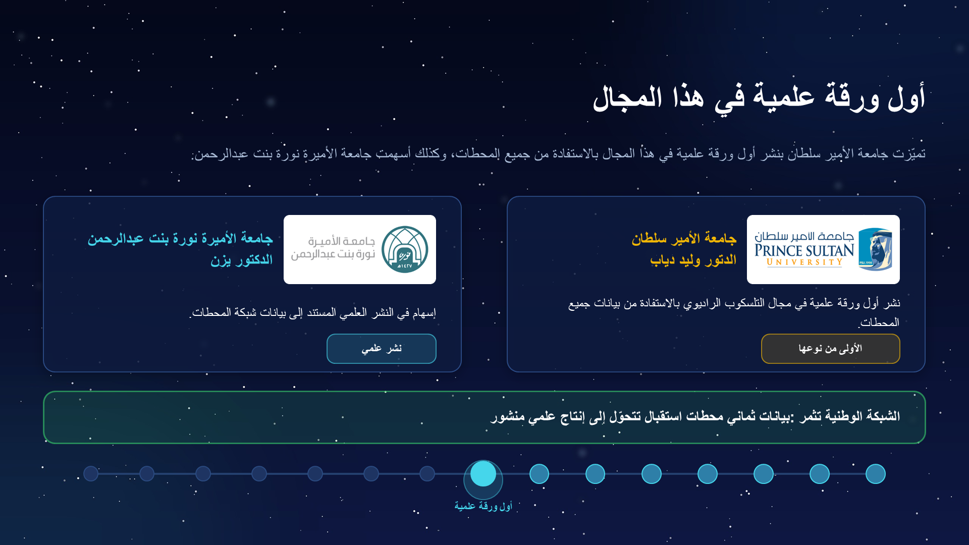
أول ورقة علمية في هذا المجال

Original PowerPoint slide 010: أول ورقة علمية في هذا المجال

تربط الشريحة بين البنية الميدانية والناتج العلمي. نشر ورقة علمية بالاستفادة من المحطات يعني أن المشروع بدأ ينتقل من البناء والتدريب إلى إنتاج معرفة قابلة للنشر والمراجعة.

تفاصيل أكثر
  • أول ورقة علمية في هذا المجال
  • تميّزت جامعة الأمير سلطان بنشر أول ورقة علمية في هذا المجال بالاستفادة من جميع المحطات، وكذلك أسهمت جامعة الأميرة نورة بنت عبدالرحمن.
  • جامعة
  • الأمير
  • سلطان
  • الدتور
  • وليد دياب
  • نشر أول ورقة علمية في مجال التلسكوب الراديوي بالاستفادة من بيانات جميع المحطات.
  • الأولى من نوعها
  • جامعة الأميرة نورة
  • بنت
  • عبدالرحمن
  • الدكتور يزن
  • إسهام في النشر العلمي المستند إلى بيانات شبكة المحطات.
  • نشر علمي
  • الشبكة الوطنية تثمر: بيانات ثماني محطات استقبال تتحوّل إلى إنتاج علمي منشور
  • أول ورقة علمية
Slide 011 / 052

قدرة محلية متكاملة: التصنيع وتحليل الإشارة

Original PowerPoint slide 011: قدرة محلية متكاملة: التصنيع وتحليل الإشارة

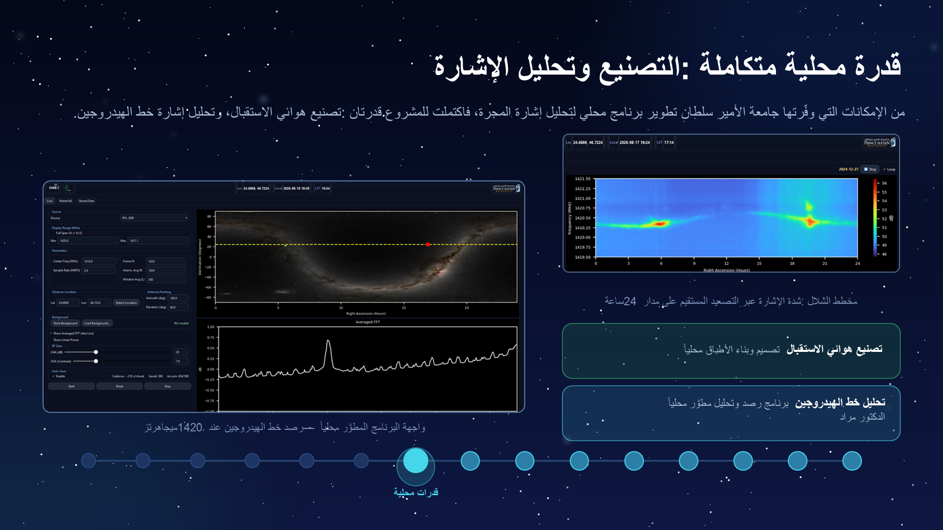
توضح الشريحة اكتمال قدرتين محليتين مترابطتين: تصنيع هوائي الاستقبال وتحليل إشارة خط الهيدروجين. واجهة البرنامج مهمة لأنها تمثل انتقال المشروع من استقبال الإشارة فقط إلى تحويلها إلى طيف قابل للفهم العلمي.

تفاصيل أكثر
  • قدرة محلية متكاملة: التصنيع وتحليل الإشارة
  • من الإمكانات التي وفّرتها جامعة الأمير سلطان تطوير برنامج محلي لتحليل إشارة المجرة، فاكتملت للمشروع قدرتان: تصنيع هوائي الاستقبال، وتحليل إشارة خط الهيدروجين.
  • واجهة البرنامج المطوَّر محلياً — رصد خط الهيدروجين عند 1420 ميجاهرتز
  • مخطط الشلال: شدة الإشارة عبر التصعيد المستقيم على مدار 24 ساعة
  • تصنيع هوائي الاستقبال
  • تصميم وبناء الأطباق محلياً
  • تحليل خط الهيدروجين
  • برنامج رصد وتحليل
  • مطوَّر
  • محلياً
  • الدكتور مراد
  • قدرات محلية
Slide 012 / 052

الطموح: نحو تلسكوب راديوي متحرك

Original PowerPoint slide 012: الطموح: نحو تلسكوب راديوي متحرك

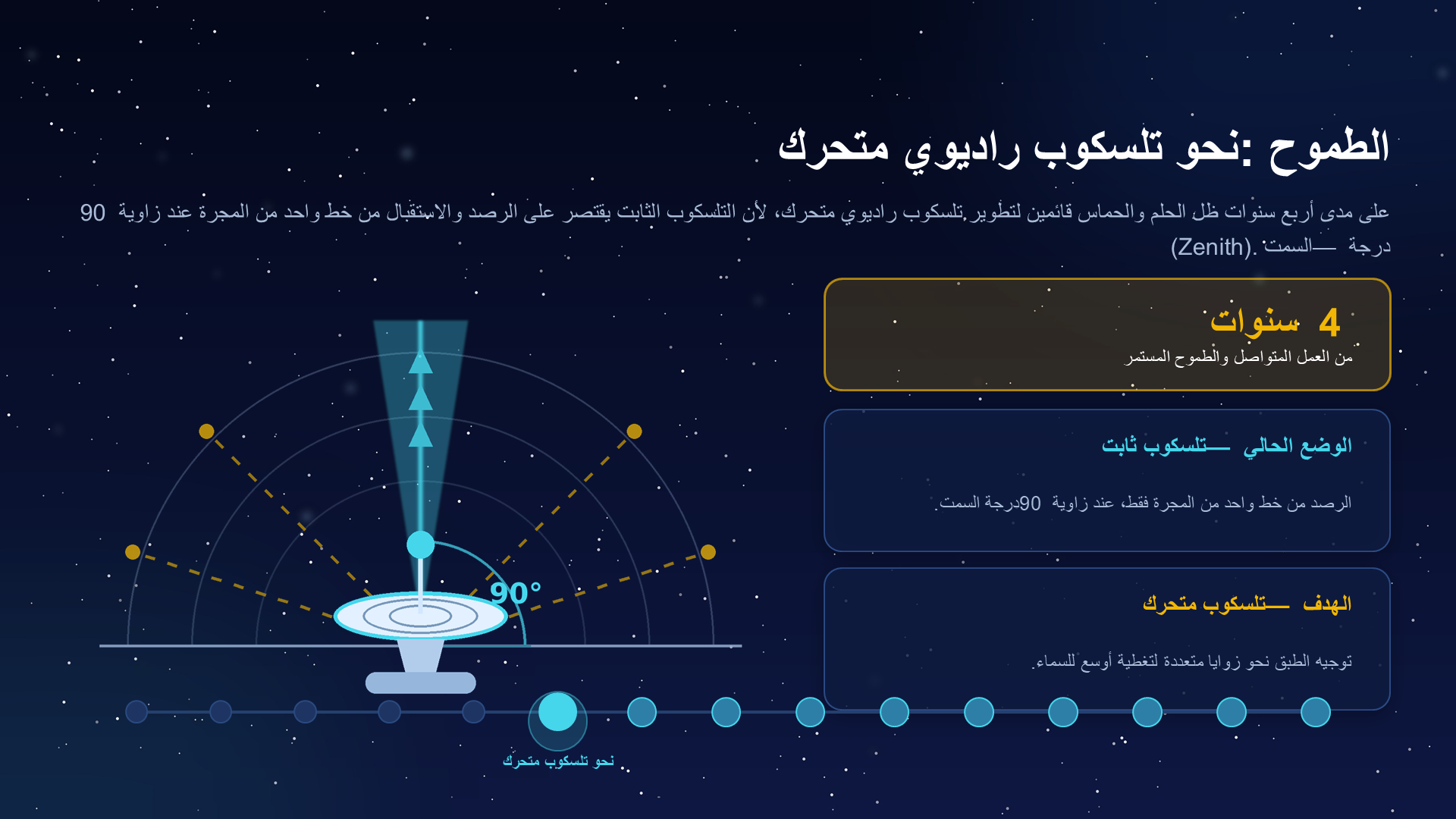
تشرح الشريحة لماذا أصبح التلسكوب المتحرك ضرورة: التلسكوب الثابت يرصد خطاً محدوداً من السماء عند السمت فقط. الحركة تعني فتح مساحة أكبر من السماء للرصد، وبالتالي الانتقال من تجربة استقبال محدودة إلى مسح فلكي أوسع.

تفاصيل أكثر
  • الطموح: نحو تلسكوب راديوي متحرك
  • على مدى أربع سنوات ظل الحلم والحماس قائمين لتطوير تلسكوب راديوي متحرك، لأن التلسكوب الثابت يقتصر على الرصد والاستقبال من خط واحد من المجرة عند زاوية 90 درجة — السمت (Zenith).
  • 4
  • سنوات
  • من العمل المتواصل والطموح المستمر
  • الوضع الحالي — تلسكوب ثابت
  • الرصد من خط واحد من المجرة فقط، عند زاوية 90
  • درجة
  • السمت
  • .
  • الهدف — تلسكوب متحرك
  • توجيه الطبق نحو زوايا متعددة لتغطية أوسع للسماء.
  • نحو تلسكوب متحرك
Slide 013 / 052

انطلاقة نظام التحكم الآلي

Original PowerPoint slide 013: انطلاقة نظام التحكم الآلي

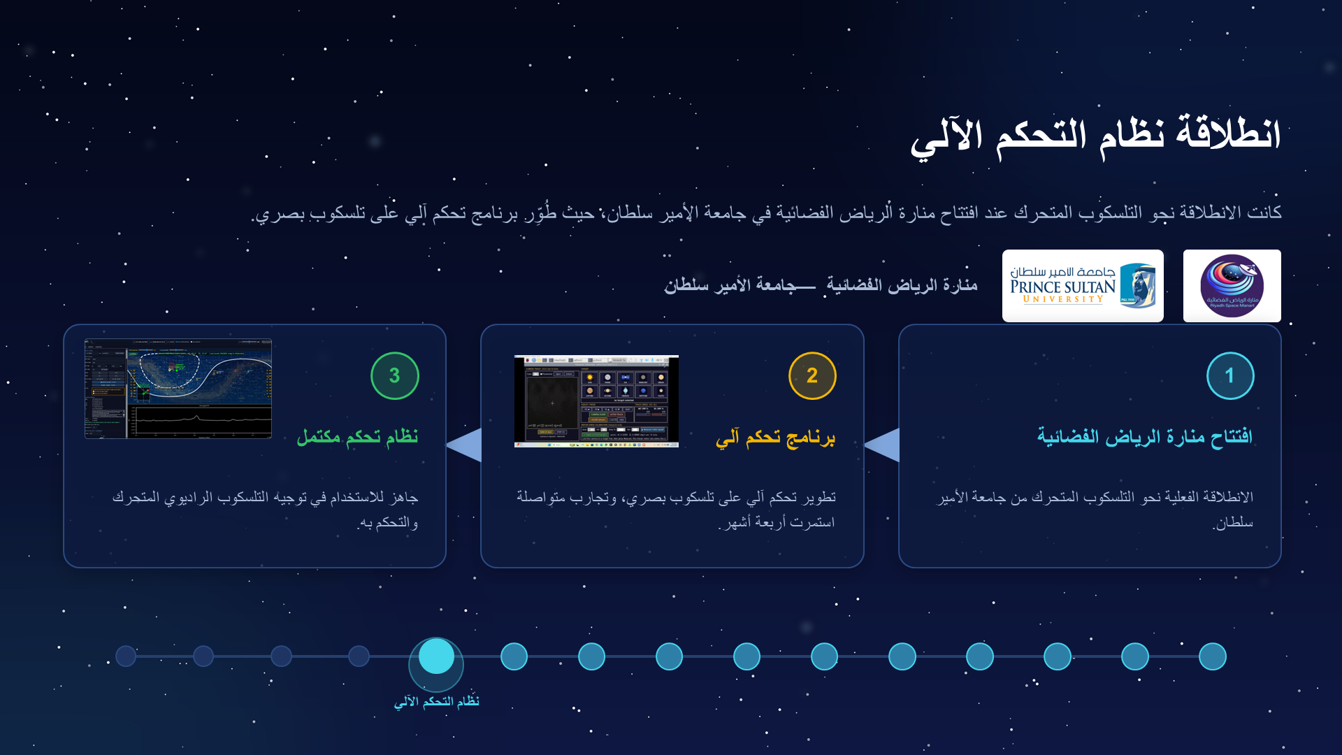
تُظهر الشريحة أن تطوير التحكم الآلي بدأ من تجربة على تلسكوب بصري في منارة الرياض الفضائية. أهمية ذلك أن مشكلة التوجيه حُلّت تدريجياً: تطوير برمجيات تحكم ثم نقل الفكرة إلى التلسكوب الراديوي المتحرك.

تفاصيل أكثر
  • انطلاقة نظام التحكم الآلي
  • كانت الانطلاقة نحو التلسكوب المتحرك عند افتتاح منارة الرياض الفضائية في جامعة الأمير سلطان، حيث طُوِّر برنامج تحكم آلي على تلسكوب بصري.
  • منارة الرياض الفضائية — جامعة الأمير سلطان
  • 1
  • افتتاح منارة الرياض الفضائية
  • الانطلاقة الفعلية نحو التلسكوب المتحرك من جامعة الأمير سلطان.
  • 2
  • برنامج تحكم آلي
  • تطوير تحكم آلي على تلسكوب بصري، وتجارب متواصلة استمرت أربعة أشهر.
  • 3
  • نظام تحكم مكتمل
  • جاهز للاستخدام في توجيه التلسكوب الراديوي المتحرك والتحكم به.
  • نظام التحكم الآلي
Slide 014 / 052

شرائح الفيبرجلاس: طبق أخف وأسهل تركيباً

Original PowerPoint slide 014: شرائح الفيبرجلاس: طبق أخف وأسهل تركيباً

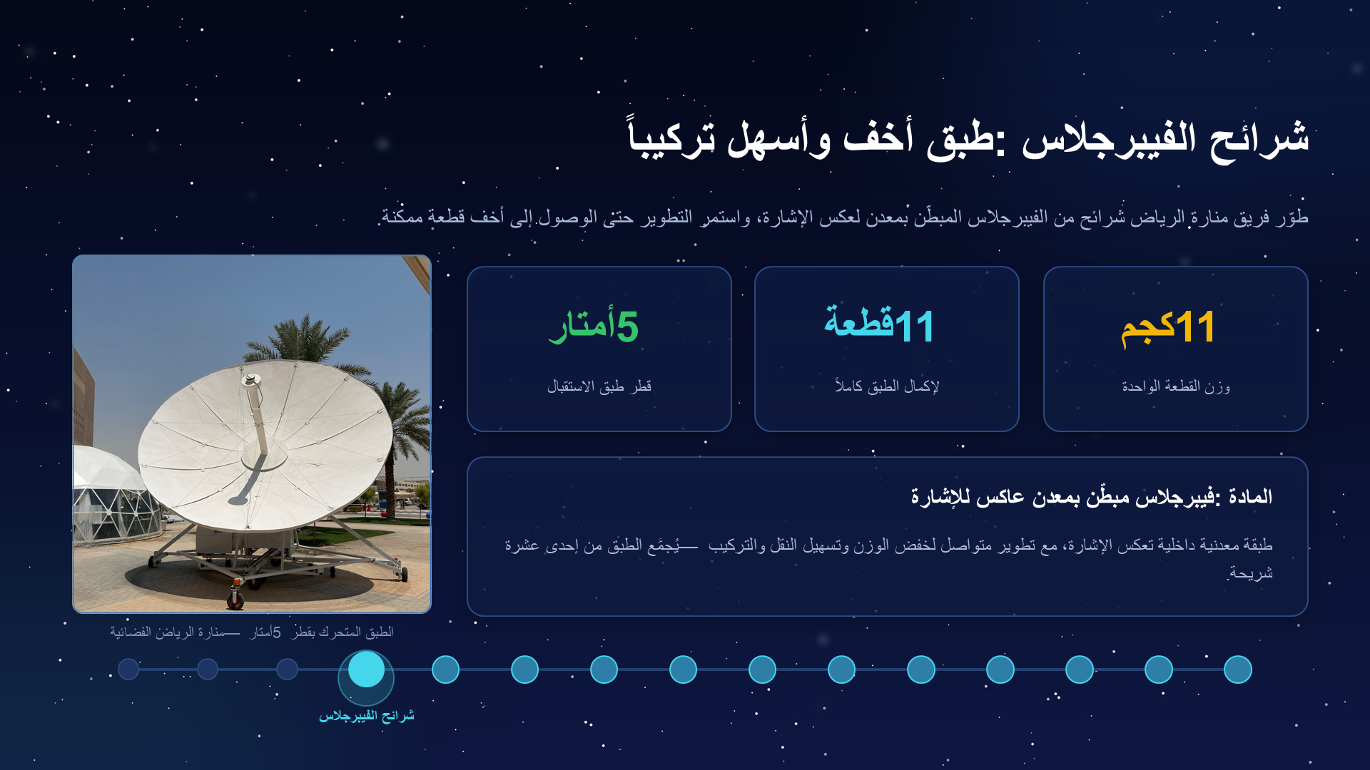
تركز الشريحة على تخفيف الطبق عبر شرائح فيبرجلاس مبطنة بمعدن عاكس. تقليل وزن كل قطعة إلى 11 كجم يجعل التركيب والحركة أكثر واقعية، لأن التلسكوب المتحرك يحتاج بنية أخف من الطبق الثابت.

تفاصيل أكثر
  • شرائح الفيبرجلاس: طبق أخف وأسهل تركيباً
  • طوّر فريق منارة الرياض شرائح من الفيبرجلاس المبطّن بمعدن لعكس الإشارة، واستمر التطوير حتى الوصول إلى أخف قطعة ممكنة.
  • الطبق المتحرك بقطر 5 أمتار — منارة الرياض الفضائية
  • 11 كجم
  • وزن القطعة الواحدة
  • 11 قطعة
  • لإكمال الطبق كاملاً
  • 5 أمتار
  • قطر طبق الاستقبال
  • المادة: فيبرجلاس مبطّن بمعدن عاكس للإشارة
  • طبقة معدنية داخلية تعكس الإشارة، مع تطوير متواصل لخفض الوزن وتسهيل النقل والتركيب — يُجمَّع الطبق من إحدى عشرة شريحة.
  • شرائح الفيبرجلاس
Slide 015 / 052

تطوير تلسكوب شراعي قابل للطوي خاص بمحطات المدارس

Original PowerPoint slide 015: تطوير تلسكوب شراعي قابل للطوي خاص بمحطات المدارس

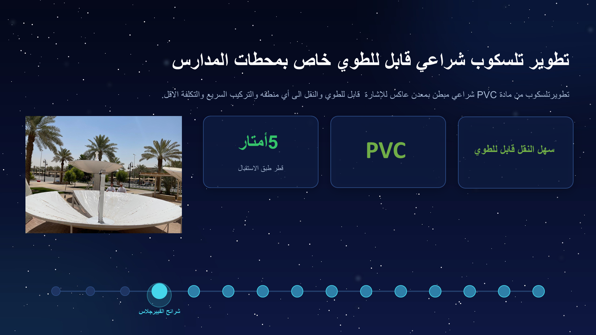
هذه الشريحة لا تتحدث عن شرائح الفيبرجلاس السابقة، بل عن مفهوم مختلف: تلسكوب شراعي قابل للطي مصنوع من PVC ومناسب لمحطات المدارس. الفكرة التعليمية هنا هي جعل الرصد الراديوي أكثر قابلية للنقل والتركيب في بيئات مدرسية، حتى لو كان أبسط من منظومة الطبق المتحرك الكبيرة.

تفاصيل أكثر
  • تطوير تلسكوب شراعي قابل للطوي خاص بمحطات المدارس
  • تطويرتلسكوب
  • من مادة
  • PVC
  • شراعي مبطن بمعدن عاكس للإشارة قابل للطوي والنقل الى أي منطقه والتركيب السريع والتكلفة الاقل
  • .
  • 5 أمتار
  • قطر طبق الاستقبال
  • شرائح الفيبرجلاس
  • PVC
  • سهل النقل قابل للطوي
Slide 016 / 052

اكتمال المنظومة: تصنيع وتحكم وتحليل

Original PowerPoint slide 016: اكتمال المنظومة: تصنيع وتحكم وتحليل

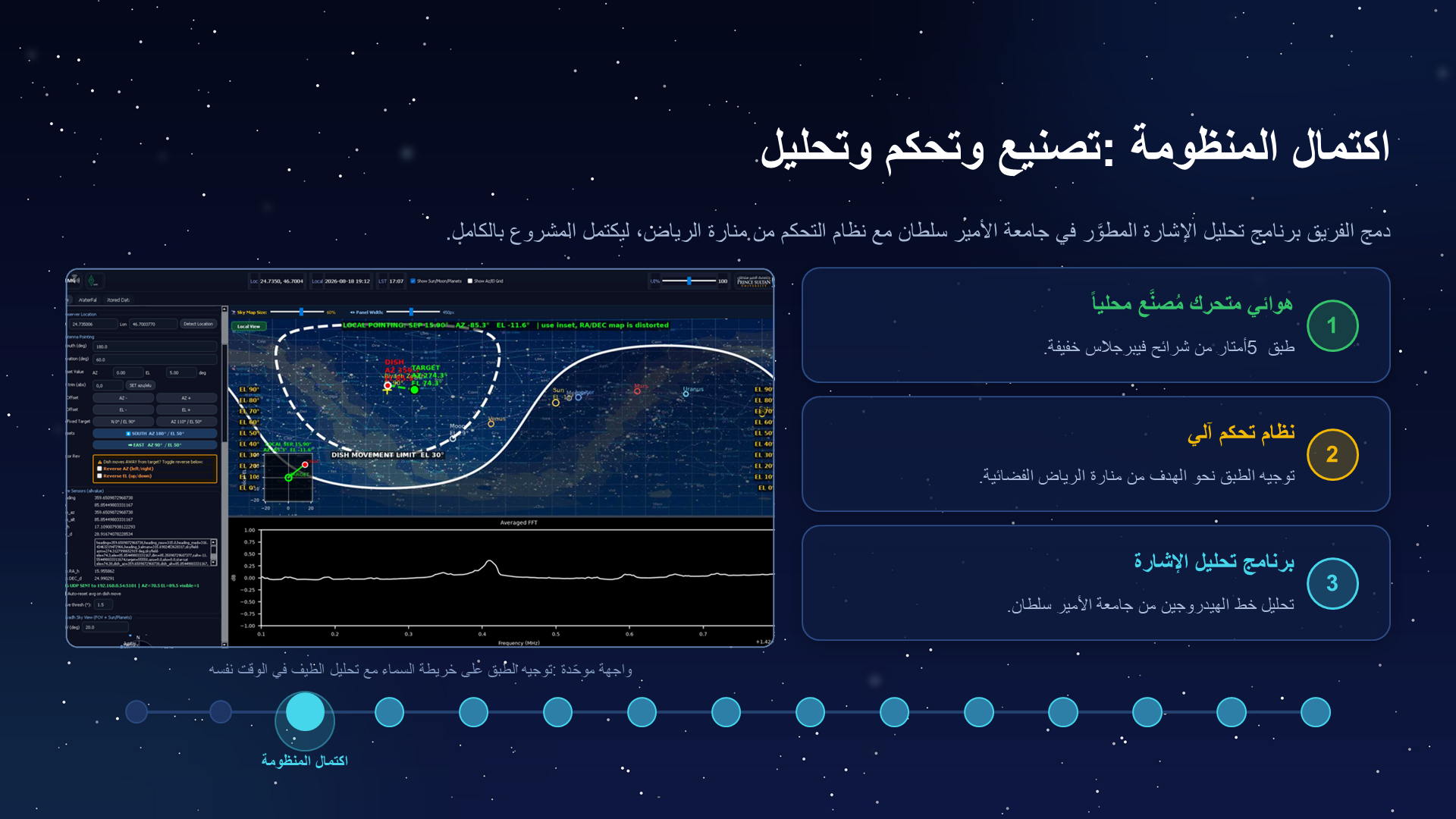
تعرض الشريحة لحظة التكامل: برنامج تحليل الإشارة من جامعة الأمير سلطان يلتقي مع نظام التحكم من منارة الرياض. عند هذه النقطة يصبح المشروع منظومة واحدة تجمع التصنيع، التوجيه، والاستقبال والتحليل بدلاً من أجزاء منفصلة.

تفاصيل أكثر
  • اكتمال المنظومة: تصنيع وتحكم وتحليل
  • دمج الفريق برنامج تحليل الإشارة المطوَّر في جامعة الأمير سلطان مع نظام التحكم من منارة الرياض، ليكتمل المشروع بالكامل.
  • واجهة موحّدة: توجيه الطبق على خريطة السماء مع تحليل الطيف في الوقت نفسه
  • 1
  • هوائي متحرك مُصنَّع محلياً
  • طبق 5 أمتار من شرائح فيبرجلاس خفيفة.
  • 2
  • نظام تحكم آلي
  • توجيه الطبق نحو الهدف من منارة الرياض الفضائية.
  • 3
  • برنامج تحليل الإشارة
  • تحليل خط الهيدروجين من جامعة الأمير سلطان.
  • اكتمال المنظومة
Slide 017 / 052

المعايرة العلمية وأولى صور المسح

Original PowerPoint slide 017: المعايرة العلمية وأولى صور المسح

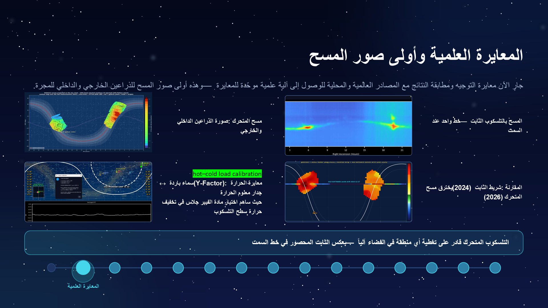
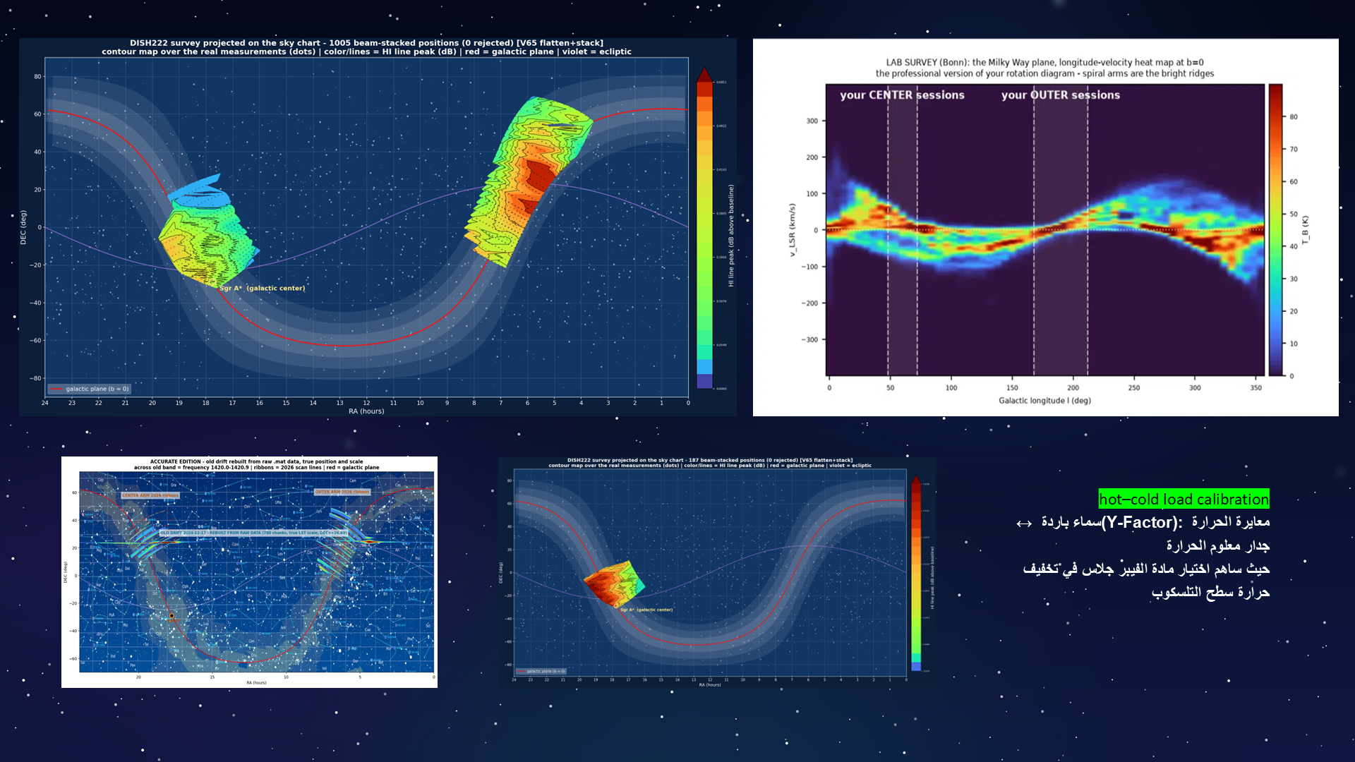
تنتقل الشريحة إلى سؤال الدقة العلمية: هل يشير التلسكوب إلى المكان الصحيح، وهل تتوافق نتائجه مع مصادر مرجعية؟ صور المسح والمعايرة توضح بداية تحويل التلسكوب المتحرك إلى أداة يمكن الوثوق بقياساتها ومقارنتها.

تفاصيل أكثر
  • المعايرة العلمية وأولى صور المسح
  • جارٍ الآن معايرة التوجيه ومطابقة النتائج مع المصادر العالمية والمحلية للوصول إلى آلية علمية موحّدة للمعايرة — وهذه أولى صور المسح للذراعين الخارجي والداخلي للمجرة.
  • المسح بالتلسكوب الثابت — خط واحد عند السمت
  • مسح المتحرك: صورة الذراعين الداخلي والخارجي
  • المقارنة: شريط الثابت (2024) يخترق مسح المتحرك (2026)
  • hot–cold load calibration
  • معايرة
  • الحرارة (Y-Factor): سماء باردة ↔ جدار
  • معلوم
  • الحرارة
  • حيث ساهم اختيار مادة
  • الفيبر
  • جلاس في تخفيف حرارة سطح التلسكوب
  • التلسكوب المتحرك قادر على تغطية أي منطقة في الفضاء آلياً — بعكس الثابت المحصور في خط السمت
  • المعايرة العلمية
Slide 018 / 052

معمل مخصص للتلسكوب الراديوي المتحرك

Original PowerPoint slide 018: معمل مخصص للتلسكوب الراديوي المتحرك

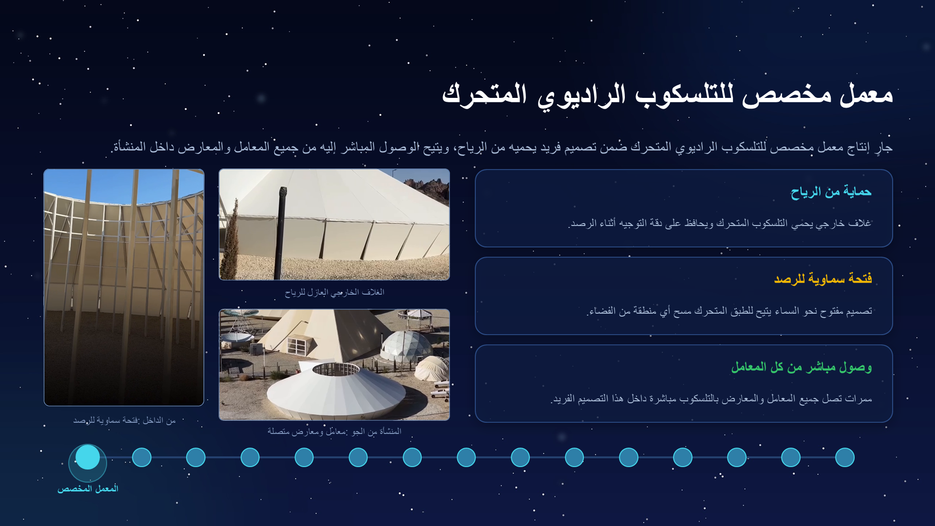
تعرض الشريحة البنية المكانية التي تحمي التلسكوب المتحرك وتجعله جزءاً من منشأة تعليمية وبحثية. الحماية من الرياح والوصول المباشر من المعامل والمعارض يربطان بين المتطلبات الهندسية واستخدامات العرض والتعليم.

تفاصيل أكثر
  • معمل مخصص للتلسكوب الراديوي المتحرك
  • جارٍ إنتاج معمل مخصص للتلسكوب الراديوي المتحرك ضمن تصميم فريد يحميه من الرياح، ويتيح الوصول المباشر إليه من جميع المعامل والمعارض داخل المنشأة.
  • من الداخل: فتحة سماوية للرصد
  • الغلاف الخارجي العازل للرياح
  • المنشأة من الجو: معامل ومعارض متصلة
  • حماية من الرياح
  • غلاف خارجي يحمي التلسكوب المتحرك ويحافظ على دقة التوجيه أثناء الرصد.
  • فتحة سماوية للرصد
  • تصميم مفتوح نحو السماء يتيح للطبق المتحرك مسح أي منطقة من الفضاء.
  • وصول مباشر من كل المعامل
  • ممرات تصل جميع المعامل والمعارض بالتلسكوب مباشرة داخل هذا التصميم الفريد.
  • المعمل المخصص
Slide 019 / 052

منظومة وطنية متكاملة للتلسكوب الراديوي

Original PowerPoint slide 019: منظومة وطنية متكاملة للتلسكوب الراديوي

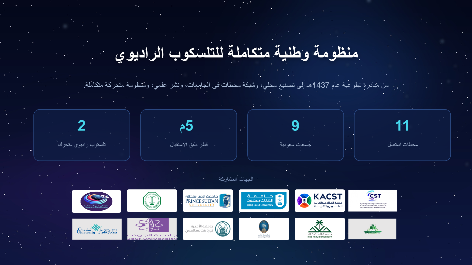
تلخص الشريحة رحلة المشروع من مبادرة تطوعية عام 1437هـ إلى شبكة محطات وتصنيع محلي ونشر علمي ومنظومة متحركة. الأرقام المعروضة في الشريحة يجب أن تُقرأ كملخص موثق من العرض نفسه، لا كزخرفة إحصائية.

تفاصيل أكثر
  • منظومة وطنية متكاملة للتلسكوب الراديوي
  • من مبادرة تطوعية عام 1437هـ إلى تصنيع محلي، وشبكة محطات في الجامعات، ونشر علمي، ومنظومة متحركة متكاملة.
  • 11
  • محطات استقبال
  • 9
  • جامعات سعودية
  • 5 م
  • قطر طبق الاستقبال
  • 2
  • تلسكوب راديوي متحرك
  • الجهات المشاركة
Slide 020 / 052

من النظام الهندسي إلى مكعب بيانات H I

Original PowerPoint slide 020: من النظام الهندسي إلى مكعب بيانات H I

هذه هي نقطة التسليم من الهندسة إلى العلم: بعد أن أصبح لدينا طبق، توجيه، مستقبل، ومعايرة، يصبح السؤال هو ما البيانات الفلكية التي نريد بناءها. الهدف المركزي يمكن كتابته هكذا \(T_B(\alpha,\delta,v_{\mathrm{LSR}})\) حيث α هو المطلع المستقيم Right Ascension، وδ هو الميل Declination، وv_LSR هي السرعة الشعاعية بالنسبة لمعيار السكون المحلي، وT_B هي درجة حرارة السطوع لانبعاث H I. بهذا تصبح المنظومة وسيلة لبناء مكعب بيانات: موضع في السماء + موضع في السماء + سرعة. والسؤال التالي هو: لماذا يكون خط H I بطول 21 سم مفيداً جداً في علم الفلك؟
تفاصيل أكثر
  • hot–cold load calibration
  • معايرة
  • الحرارة (Y-Factor): سماء باردة ↔ جدار
  • معلوم
  • الحرارة
  • حيث ساهم اختيار مادة
  • الفيبر
  • جلاس في تخفيف حرارة سطح التلسكوب
Slide 021 / 052

Why Is the 21 cm Line Important in Astronomy?

Original PowerPoint slide 021: Why Is the 21 cm Line Important in Astronomy?

Understanding this slide

This slide begins the science part of the lecture. It shifts the reader from the telescope as an engineered system to the physical signal it is built to observe: the H I 21-cm line from neutral atomic hydrogen.

Extracted slide text
  • Why Is the 21 cm Line Important in Astronomy?
  • Hyperfine hydrogen emission: physics, calibration, and observation workflow
Slide 022 / 052

Hydrogen: The Most Common Element

Original PowerPoint slide 022: Hydrogen: The Most Common Element

Understanding this slide

Hydrogen is the most abundant element, and cold hydrogen clouds are often faint or invisible in ordinary optical light. The 21-cm line gives radio telescopes a way to detect that otherwise hidden material.

Extracted slide text
  • Hydrogen: The Most Common Element
  • • Hydrogen is the most common element in the universe.
  • • Cold hydrogen clouds are often not bright in visible light.
  • • But they can emit the 21 cm radio line.
  • • This makes cold, dark gas directly observable.
Slide 023 / 052

What Astronomers Study with the 21 cm Line

Original PowerPoint slide 023: What Astronomers Study with the 21 cm Line

Understanding this slide

The slide lists the scientific payoff of 21-cm observations: Galactic gas distribution, spiral structure, radial motion and Galactic rotation, interstellar clouds, and H I in external galaxies. In other words, the line is not just a detection tool; it is a tracer of structure and motion.

Extracted slide text
  • What Astronomers Study with the 21 cm Line
  • • Spiral arms of galaxies
  • • Rotation of the Milky Way
  • • Gas clouds between stars
  • • Structure of other galaxies
  • • Dark matter effects through galaxy rotation curves
  • • Early universe hydrogen
Slide 024 / 052

Seeing Through Dust

Original PowerPoint slide 024: Seeing Through Dust

Understanding this slide

Radio waves at 21 cm can pass through dust far better than visible light. This is why H I observations reveal obscured parts of the Milky Way, including gas and spiral structure that optical images may hide.

Extracted slide text
  • Seeing Through Dust
  • • Radio waves with wavelength 21 cm pass through dust better than visible light.
  • • They therefore reveal hidden regions of galaxies.
  • • Obscured spiral structure and inner-galaxy gas become accessible.
Slide 025 / 052

Boltzmann State Populations

Original PowerPoint slide 025: Boltzmann State Populations

Understanding this slide

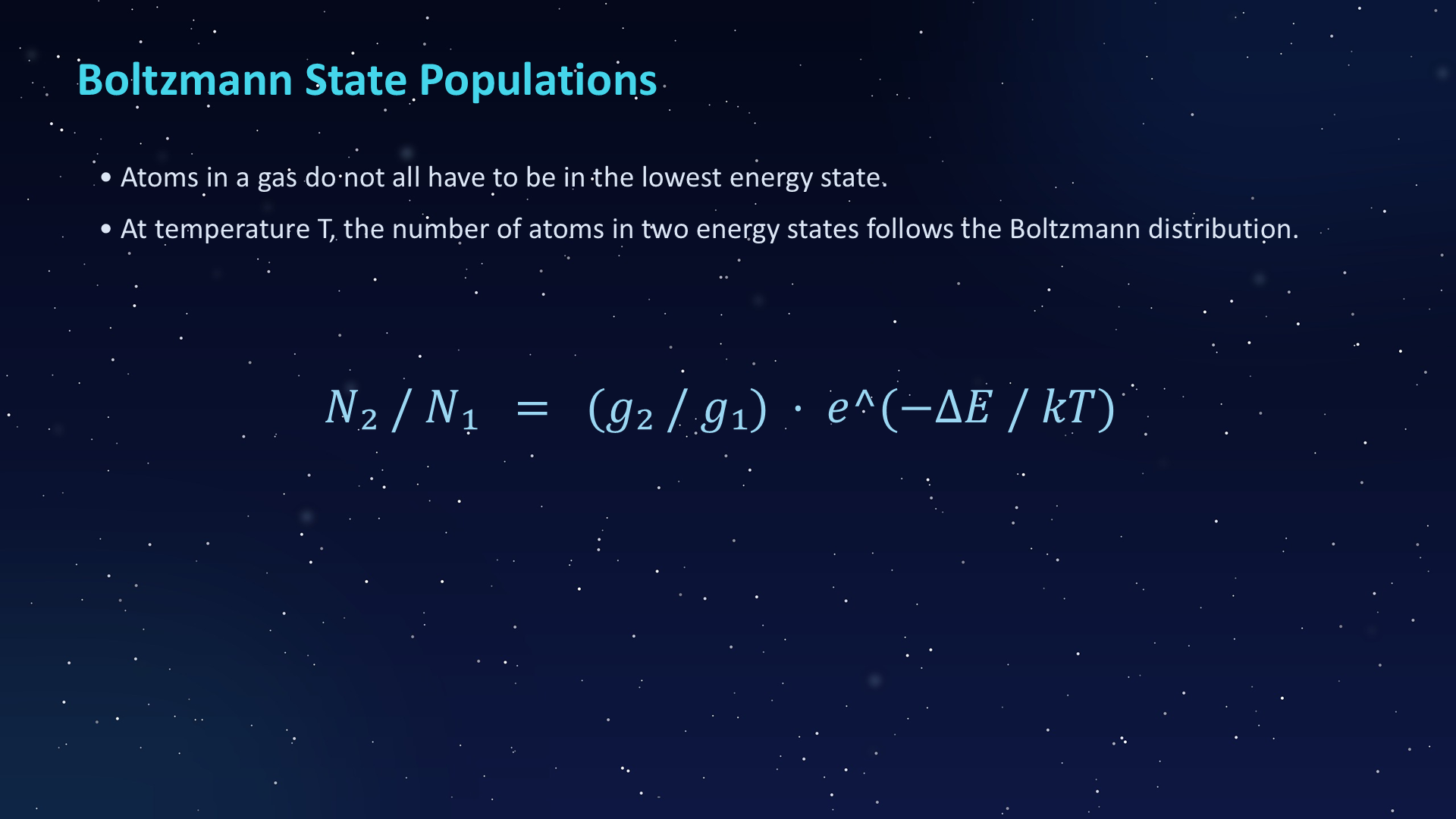
This slide introduces the population physics behind the line. The Boltzmann relation \[\frac{N_2}{N_1}=\frac{g_2}{g_1}\exp(-\frac{\Delta E}{kT})\] tells us how atoms distribute between energy states at temperature T, which prepares the reader for the hydrogen hyperfine states.

Extracted slide text
  • Boltzmann State Populations
  • • Atoms in a gas do not all have to be in the lowest energy state.
  • • At temperature T, the number of atoms in two energy states follows the Boltzmann distribution.
Slide 026 / 052

Definition of Terms

Original PowerPoint slide 026: Definition of Terms

Understanding this slide

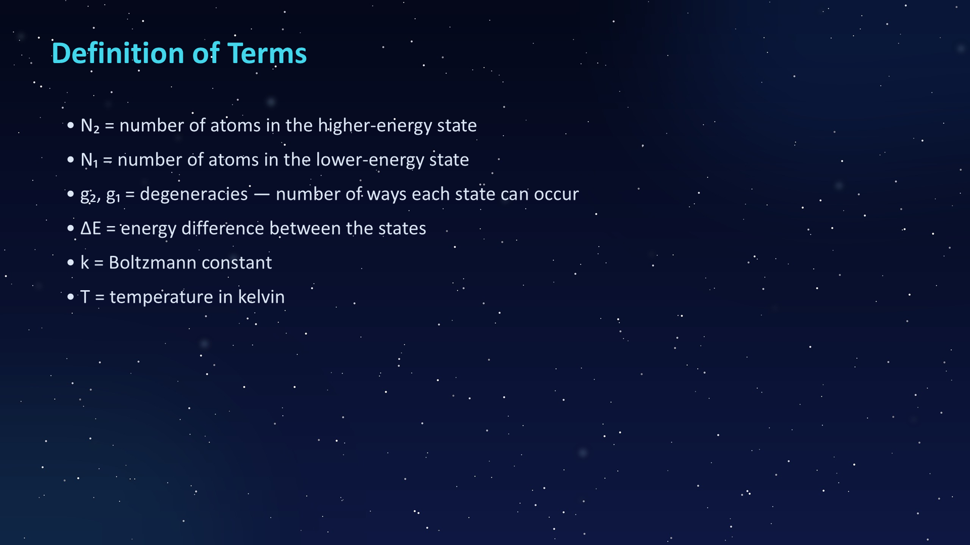
The slide defines the symbols used in the population ratio: upper- and lower-state atom numbers and their degeneracies. Getting these terms clear matters because the 21-cm line depends on the relative occupation of two very closely spaced hyperfine states.

Extracted slide text
  • Definition of Terms
  • • N₂ = number of atoms in the higher-energy state
  • • N₁ = number of atoms in the lower-energy state
  • • g₂, g₁ = degeneracies — number of ways each state can occur
  • • ΔE = energy difference between the states
  • • k = Boltzmann constant
  • • T = temperature in kelvin
Slide 027 / 052

Hydrogen Hyperfine States

Original PowerPoint slide 027: Hydrogen Hyperfine States

Understanding this slide

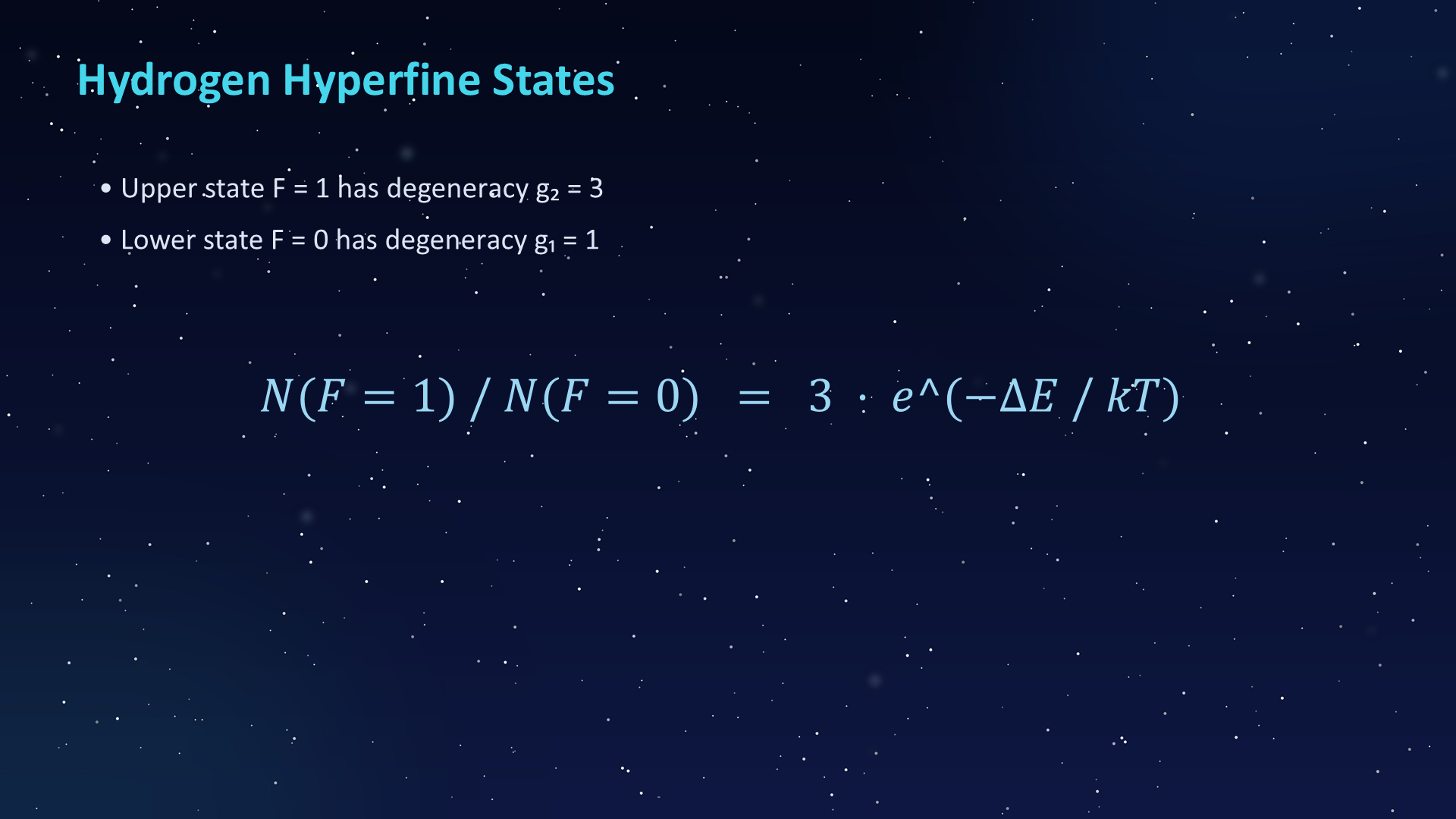
Hydrogen’s upper hyperfine state has three allowed orientations, while the lower state has one. That 3:1 degeneracy is why, in the high-temperature limit, many more atoms occupy the upper state even though the energy difference is tiny.

Extracted slide text
  • Hydrogen Hyperfine States
  • • Upper state F = 1 has degeneracy g₂ = 3
  • • Lower state F = 0 has degeneracy g₁ = 1
Slide 028 / 052

The High-Temperature Limit

Original PowerPoint slide 028: The High-Temperature Limit

Understanding this slide

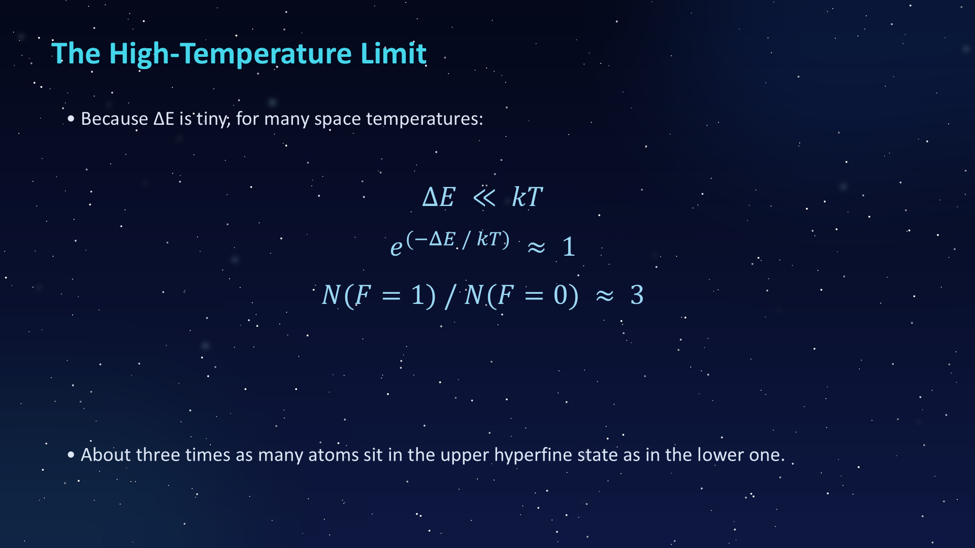
Because the hyperfine energy gap is extremely small, many interstellar environments behave like the high-temperature limit for this transition. The result is a nearly 3:1 upper-to-lower population ratio, which helps make the line observable at astronomical scales.

Extracted slide text
  • The High-Temperature Limit
  • • Because ΔE is tiny, for many space temperatures:
  • • About three times as many atoms sit in the upper hyperfine state as in the lower one.
Slide 029 / 052

Example: Interstellar Hydrogen at T = 100 K

Original PowerPoint slide 029: Example: Interstellar Hydrogen at T = 100 K

Understanding this slide

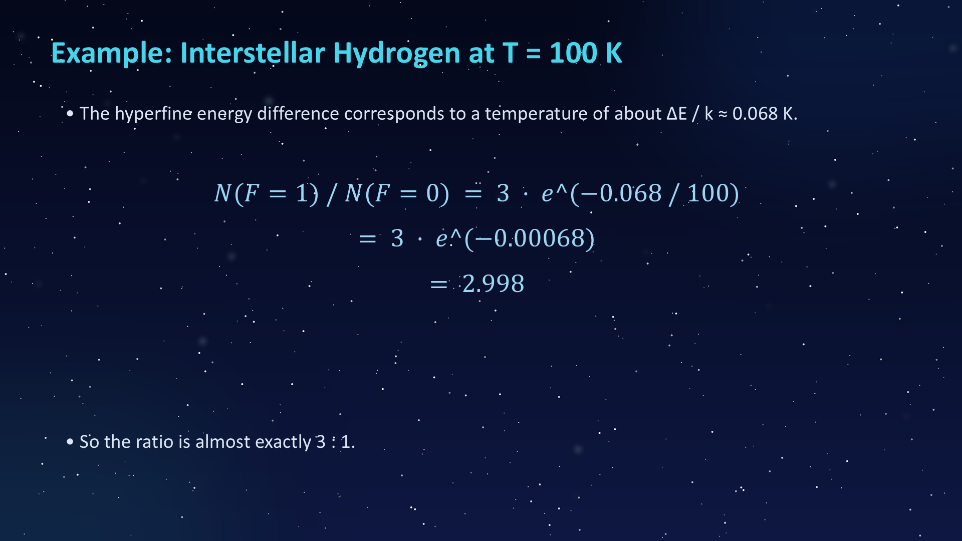
At T = 100 K, the hyperfine energy difference is tiny compared with thermal energy. The example shows why the population ratio is almost exactly 3:1 in typical cold interstellar hydrogen, reinforcing the high-temperature approximation.

Extracted slide text
  • Example: Interstellar Hydrogen at T = 100 K
  • • The hyperfine energy difference corresponds to a temperature of about ΔE / k ≈ 0.068 K.
  • • So the ratio is almost exactly 3 : 1.
Slide 030 / 052

Einstein Coefficients

Original PowerPoint slide 030: Einstein Coefficients

Understanding this slide

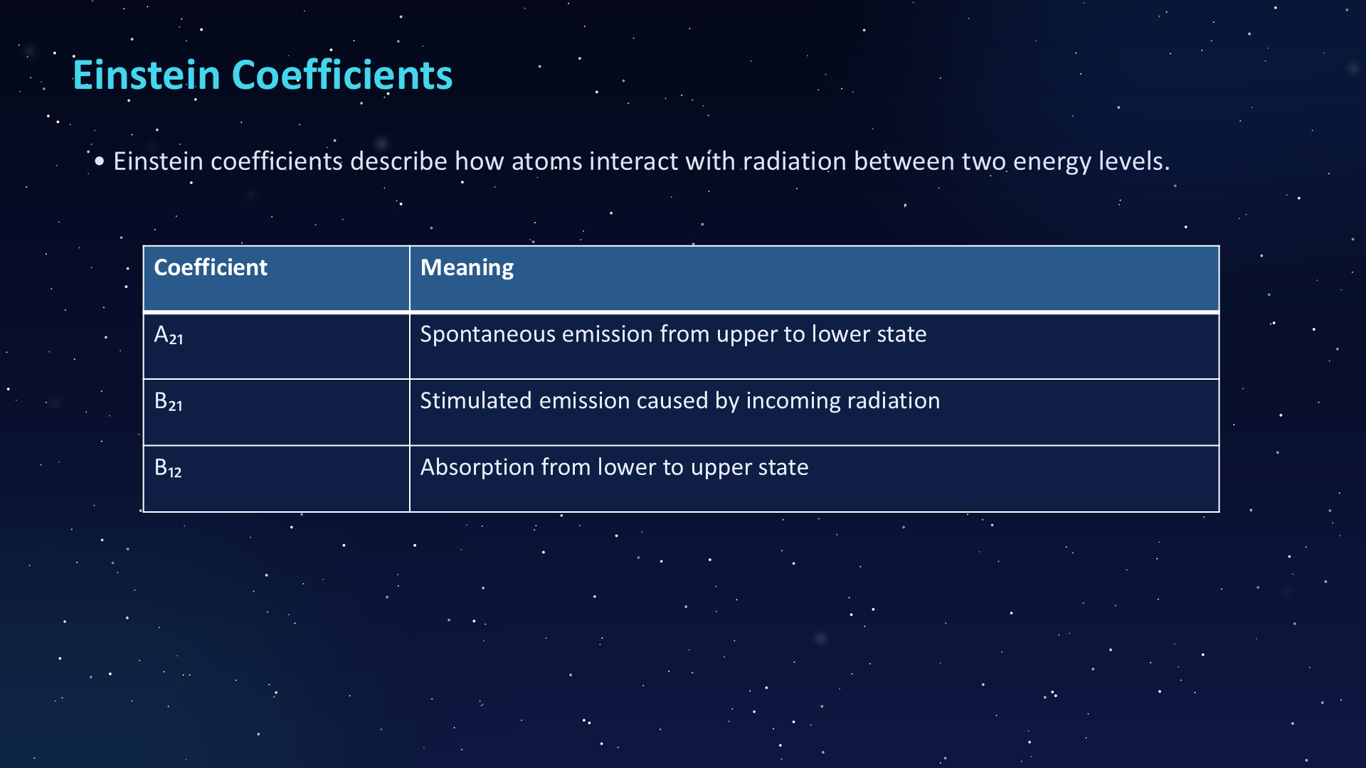
Einstein coefficients are bookkeeping constants for how atoms interact with radiation: absorption, stimulated emission, and spontaneous emission. The deck introduces them because the 21-cm line is governed by a very small spontaneous-emission probability.

Extracted slide text
  • Einstein Coefficients
  • • Einstein coefficients describe how atoms interact with radiation between two energy levels.
  • Coefficient
  • Meaning
  • A₂₁
  • Spontaneous emission from upper to lower state
  • B₂₁
  • Stimulated emission caused by incoming radiation
  • B₁₂
  • Absorption from lower to upper state
Slide 031 / 052

Spontaneous Emission: A₂₁

Original PowerPoint slide 031: Spontaneous Emission: A₂₁

Understanding this slide

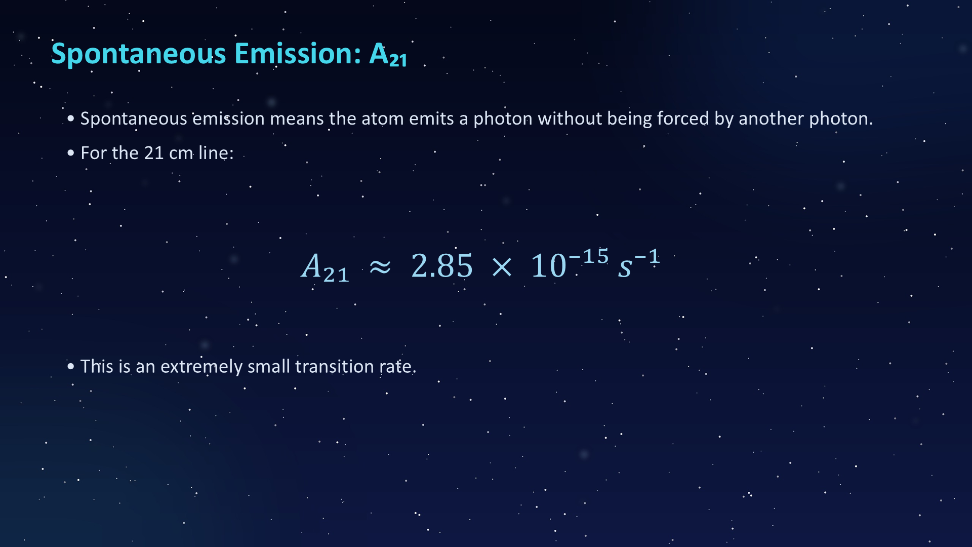
The coefficient \(A_{21}\approx2.85\times10^{-15}\,\mathrm{s^{-1}}\) is the probability per second that an atom in the upper hyperfine state emits a 21-cm photon spontaneously. Its extremely small value means an individual atom rarely emits, which naturally leads to Slide 32’s long upper-state lifetime.

Extracted slide text
  • Spontaneous Emission: A₂₁
  • • Spontaneous emission means the atom emits a photon without being forced by another photon.
  • • For the 21 cm line:
  • • This is an extremely small transition rate.
Slide 032 / 052

Lifetime of the Upper State

Original PowerPoint slide 032: Lifetime of the Upper State

Understanding this slide

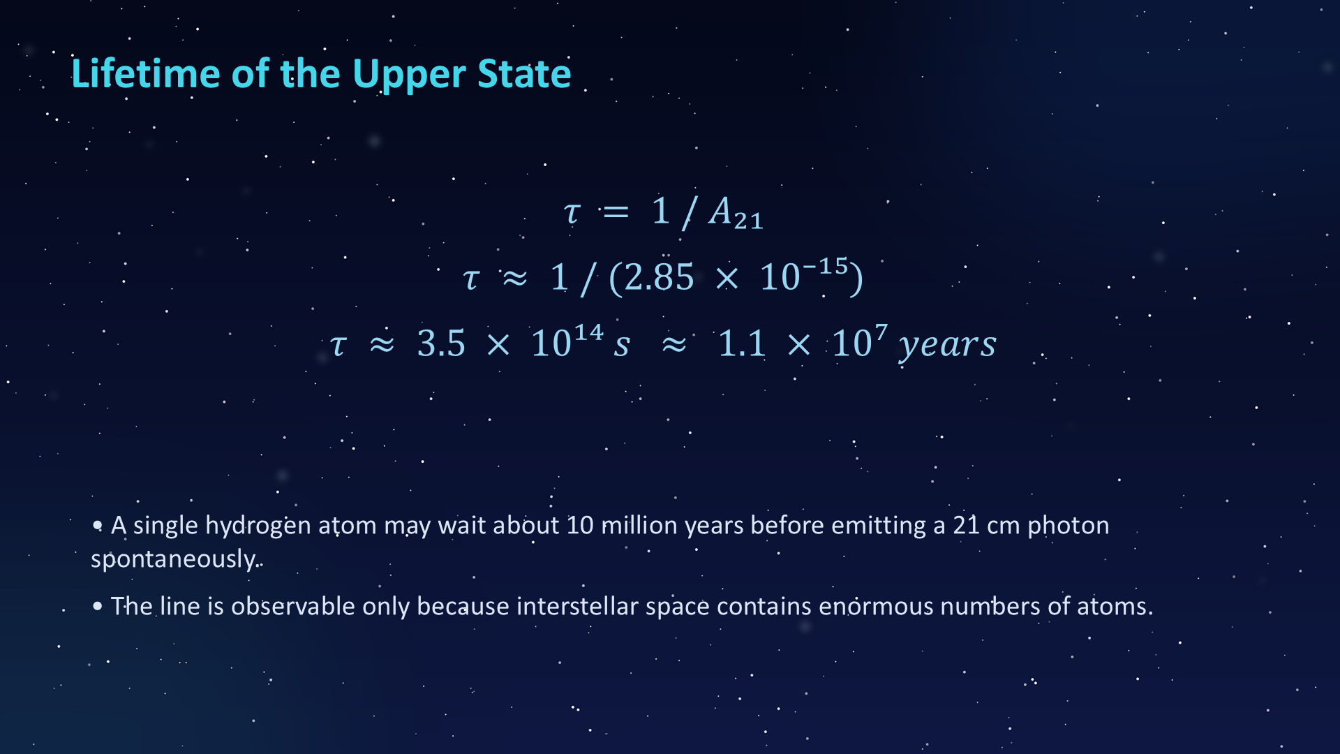
A lifetime of roughly ten million years sounds too long to be useful, but the interstellar medium contains enormous numbers of hydrogen atoms. The line is observable because rare emission events become abundant when summed over vast clouds of gas.

Extracted slide text
  • Lifetime of the Upper State
  • • A single hydrogen atom may wait about 10 million years before emitting a 21 cm photon spontaneously.
  • • The line is observable only because interstellar space contains enormous numbers of atoms.
Slide 033 / 052

Example Hydrogen Observation Workflow (1–5)

Original PowerPoint slide 033: Example Hydrogen Observation Workflow (1–5)

Understanding this slide

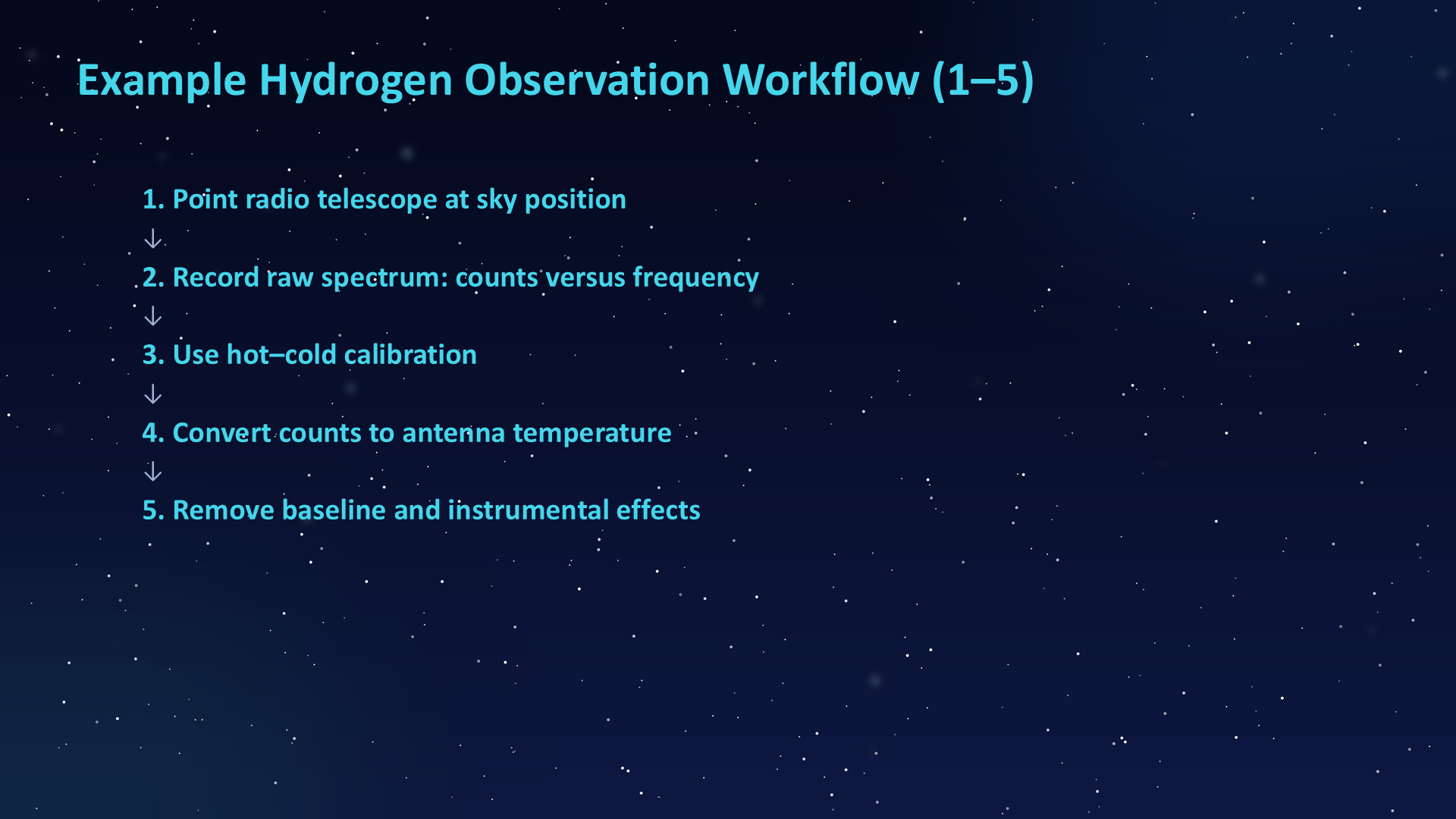
The workflow starts with a pointing and a raw spectrum. At this stage the telescope is not yet producing a final map; it is collecting frequency-channel measurements that must still be calibrated and interpreted.

Extracted slide text
  • Example Hydrogen Observation Workflow (1–5)
  • 1. Point radio telescope at sky position
  • 2. Record raw spectrum: counts versus frequency
  • 3. Use hot–cold calibration
  • 4. Convert counts to antenna temperature
  • 5. Remove baseline and instrumental effects
Slide 034 / 052

Example Hydrogen Observation Workflow (6–9)

Original PowerPoint slide 034: Example Hydrogen Observation Workflow (6–9)

Understanding this slide

This second workflow slide completes the transformation from raw frequency measurements to astronomical velocity products. Frequency shifts become Doppler velocities, and LSR correction puts those velocities into a frame useful for Galactic comparison.

Extracted slide text
  • Example Hydrogen Observation Workflow (6–9)
  • 6. Convert frequency to Doppler velocity
  • 7. Apply LSR correction
  • 8. Correct for beam efficiency and pointing errors
  • 9. Report brightness temperature versus LSR velocity
Slide 035 / 052

Step 1: Point the Telescope at a Sky Position

Original PowerPoint slide 035: Step 1: Point the Telescope at a Sky Position

Understanding this slide

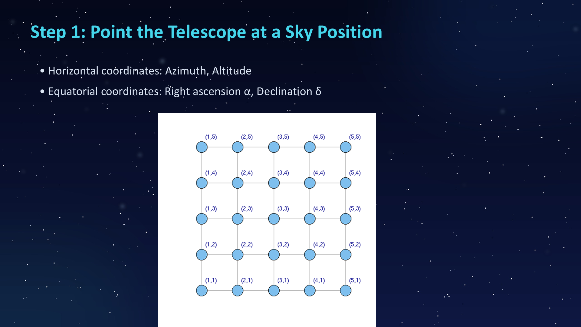
Azimuth and Altitude are local horizon coordinates: they describe where the telescope mount points from a specific site at a specific time. Right Ascension α and Declination δ are celestial coordinates fixed on the sky, so the control system must convert target RA/Dec into the local azimuth/altitude commands needed by the telescope.

Extracted slide text
  • Step 1: Point the Telescope at a Sky Position
  • • Horizontal coordinates: Azimuth, Altitude
  • • Equatorial coordinates: Right ascension α, Declination δ
Slide 036 / 052

Step 2: Record the Raw Spectrum

Original PowerPoint slide 036: Step 2: Record the Raw Spectrum

Understanding this slide

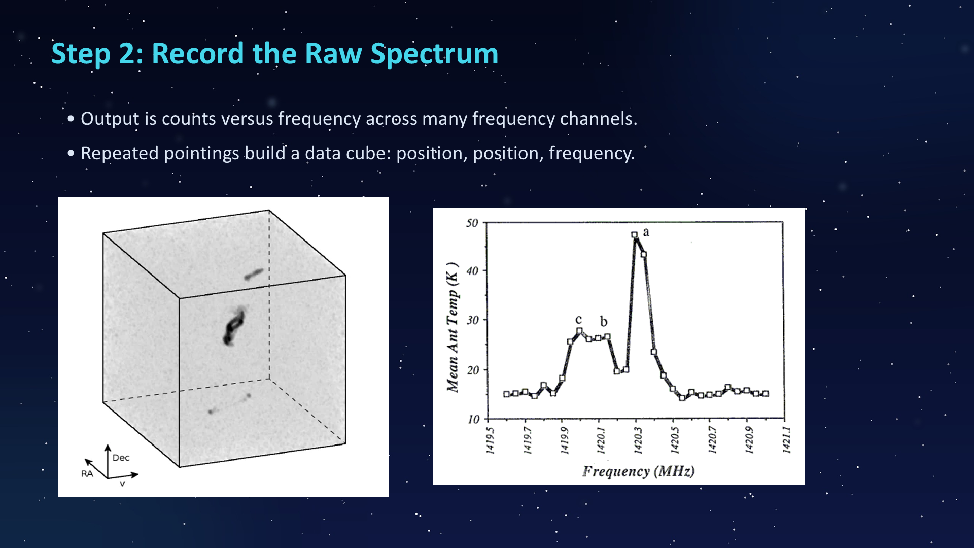
This slide is deliberately still early in the measurement chain. The receiver output is counts versus frequency across spectral channels; repeated pointings begin to form position × position × frequency measurements before calibration and velocity conversion turn them into the final science cube.

Extracted slide text
  • Step 2: Record the Raw Spectrum
  • • Output is counts versus frequency across many frequency channels.
  • • Repeated pointings build a data cube: position, position, frequency.
Slide 037 / 052

Antenna Temperature

Original PowerPoint slide 037: Antenna Temperature

Understanding this slide

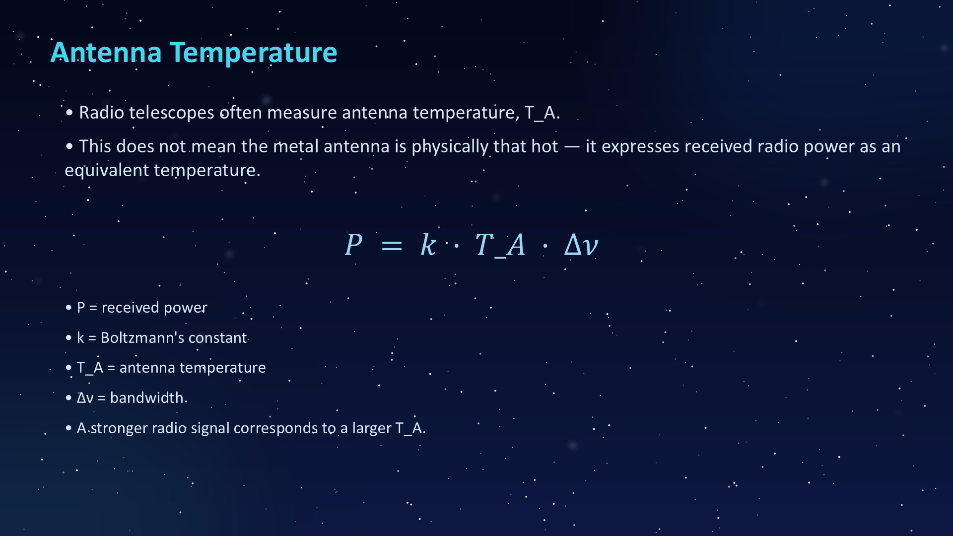
Antenna temperature is an equivalent way to express received radio power; it is not the physical temperature of the metal dish. The relation \[P=kT_A\Delta\nu\] says that received power depends on Boltzmann’s constant, antenna temperature T_A, and bandwidth Δν.

Extracted slide text
  • Antenna Temperature
  • • Radio telescopes often measure antenna temperature, T_A.
  • • This does not mean the metal antenna is physically that hot — it expresses received radio power as an equivalent temperature.
  • • P = received power
  • • k = Boltzmann's constant
  • • T_A = antenna temperature
  • • Δν = bandwidth
  • • A stronger radio signal corresponds to a larger T_A.
Slide 038 / 052

Step 3: Hot–Cold Calibration

Original PowerPoint slide 038: Step 3: Hot–Cold Calibration

Understanding this slide

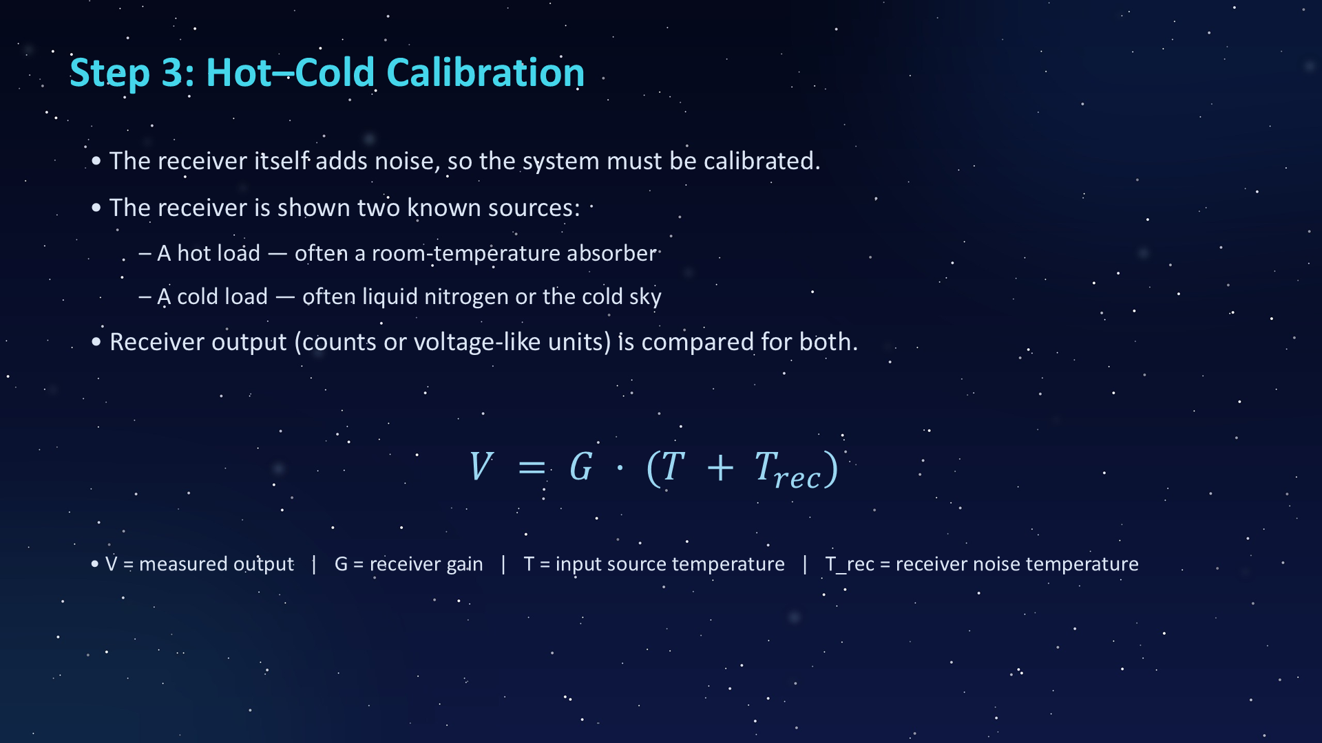
Hot–cold calibration compares receiver output for known warm and cold references. The simple receiver model \[V=G(T+T_{\mathrm{rec}})\] says measured voltage or counts V are set by gain G multiplying the input temperature plus the receiver’s own noise temperature T_rec.

Extracted slide text
  • Step 3: Hot–Cold Calibration
  • • The receiver itself adds noise, so the system must be calibrated.
  • • The receiver is shown two known sources:
  • – A hot load — often a room-temperature absorber
  • – A cold load — often liquid nitrogen or the cold sky
  • • Receiver output (counts or voltage-like units) is compared for both.
  • • V = measured output | G = receiver gain | T = input source temperature | T_rec = receiver noise temperature
Slide 039 / 052

Calibration Equations

Original PowerPoint slide 039: Calibration Equations

Understanding this slide

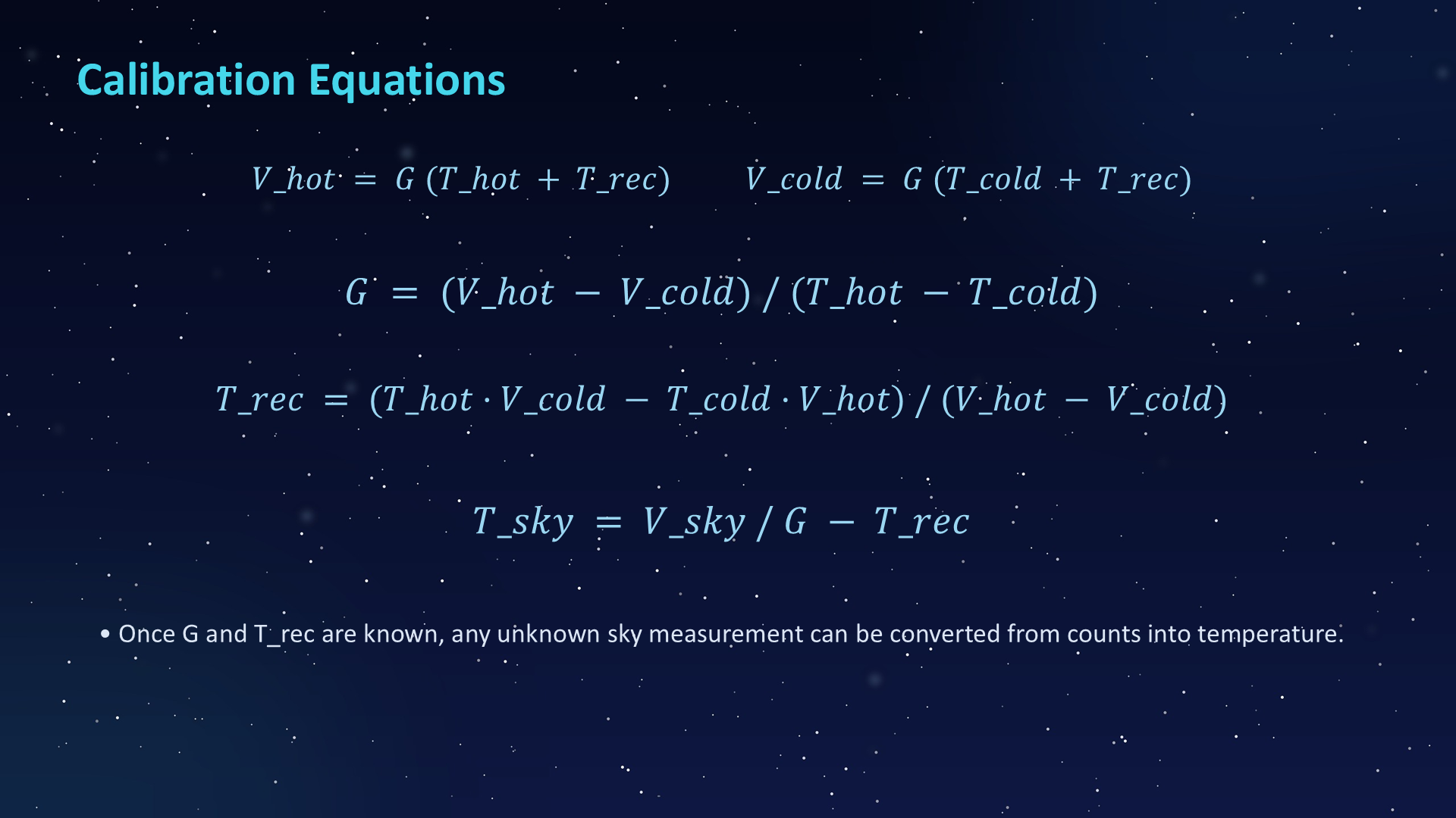
This slide is where the hot and cold measurements become calibration constants. By observing two known temperatures, the system solves for gain G and receiver temperature T_rec, allowing an unknown sky measurement to be converted from counts into temperature.

Extracted slide text
  • Calibration Equations
  • • Once G and T_rec are known, any unknown sky measurement can be converted from counts into temperature.
Slide 040 / 052

Step 5: Remove Baseline and Instrumental Effects

Original PowerPoint slide 040: Step 5: Remove Baseline and Instrumental Effects

Understanding this slide

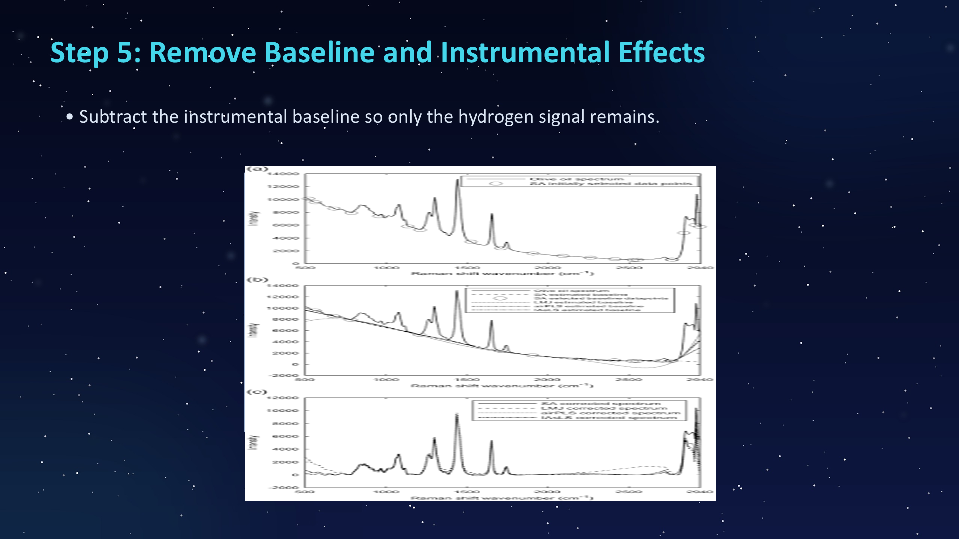
Baseline removal subtracts the slowly varying instrumental response from the measured spectrum so that the H I line can be distinguished from receiver slope and bandpass structure. The baseline should represent the instrumental/background trend rather than the astronomical line itself.

Extracted slide text
  • Step 5: Remove Baseline and Instrumental Effects
  • • Subtract the instrumental baseline so only the hydrogen signal remains.
  • [ Insert baseline-removal figure ]
Slide 041 / 052

Brightness Temperature

Original PowerPoint slide 041: Brightness Temperature

Understanding this slide

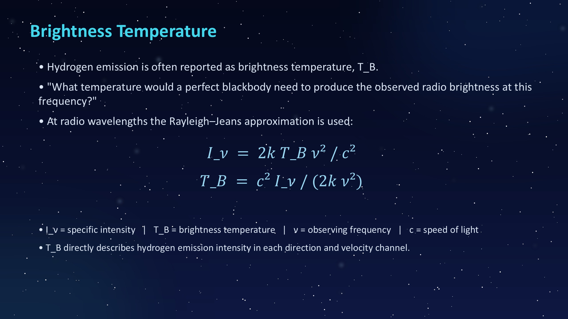
Brightness temperature T_B expresses radio intensity as the temperature a blackbody would need to have to produce the same specific intensity at that frequency. In the Rayleigh–Jeans limit the relationship is \[I_\nu=\frac{2kT_B\nu^2}{c^2}\], which is why H I maps are commonly shown in kelvin.

Extracted slide text
  • Brightness Temperature
  • • Hydrogen emission is often reported as brightness temperature, T_B.
  • • "What temperature would a perfect blackbody need to produce the observed radio brightness at this frequency?"
  • • At radio wavelengths the Rayleigh–Jeans approximation is used:
  • • I_ν = specific intensity | T_B = brightness temperature | ν = observing frequency | c = speed of light
  • • T_B directly describes hydrogen emission intensity in each direction and velocity channel.
Slide 042 / 052

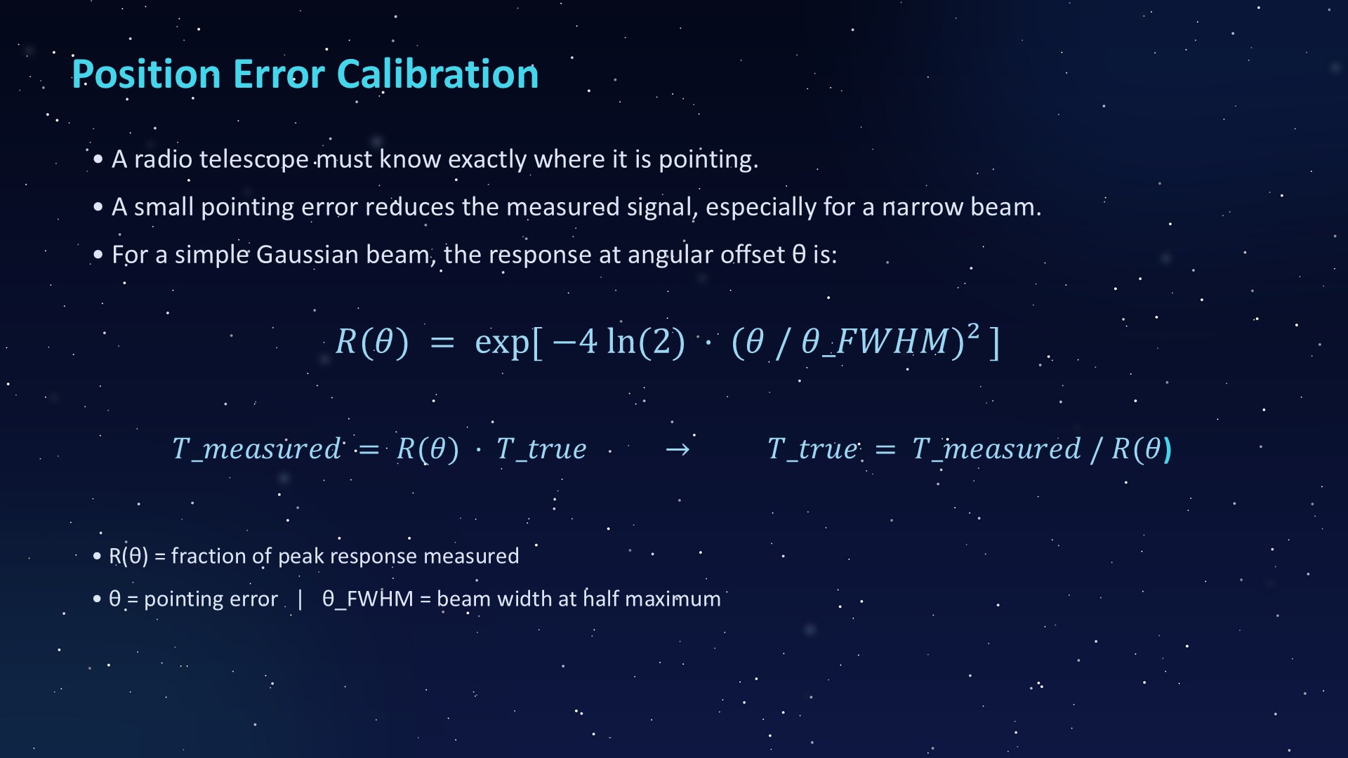
Position Error Calibration

Original PowerPoint slide 042: Position Error Calibration

Understanding this slide

A pointing error moves the source away from the beam center and reduces the measured amplitude. For a Gaussian beam the response follows \[R(\theta)=\exp[-4\ln 2(\theta/\theta_{\mathrm{FWHM}})^2]\], so the penalty depends on the pointing offset θ relative to the beam width θ_FWHM.

Extracted slide text
  • Position Error Calibration
  • • A radio telescope must know exactly where it is pointing.
  • • A small pointing error reduces the measured signal, especially for a narrow beam.
  • • For a simple Gaussian beam, the response at angular offset θ is:
  • )
  • • R(θ) = fraction of peak response measured
  • • θ = pointing error | θ_FWHM = beam width at half maximum
Slide 043 / 052

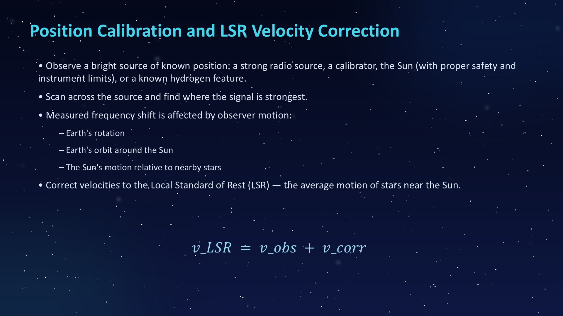
Position Calibration and LSR Velocity Correction

Original PowerPoint slide 043: Position Calibration and LSR Velocity Correction

Understanding this slide

v_obs is the velocity inferred directly from the measured frequency shift at the observatory. v_LSR is the corrected velocity after accounting for Earth’s rotation, Earth’s orbit, and the Sun’s motion relative to nearby stars, which is necessary before comparing Galactic gas velocities.

Extracted slide text
  • Position Calibration and LSR Velocity Correction
  • • Observe a bright source of known position: a strong radio source, a calibrator, the Sun (with proper safety and instrument limits), or a known hydrogen feature.
  • • Scan across the source and find where the signal is strongest.
  • • Measured frequency shift is affected by observer motion:
  • – Earth's rotation
  • – Earth's orbit around the Sun
  • – The Sun's motion relative to nearby stars
  • • Correct velocities to the Local Standard of Rest (LSR) — the average motion of stars near the Sun.
Slide 044 / 052

Understanding Moment Maps

Original PowerPoint slide 044: Understanding Moment Maps

Understanding this slide

Moment maps are a way to summarize a spectral data cube into maps that are easier to inspect. This slide introduces moments 0 through 4 as different summaries of the line profile at each sky position.

Extracted slide text
  • Understanding Moment Maps
  • Moment 0 to Moment 4
  • H I 21 cm astronomy
  • From spectral data cubes to physical maps
Slide 045 / 052

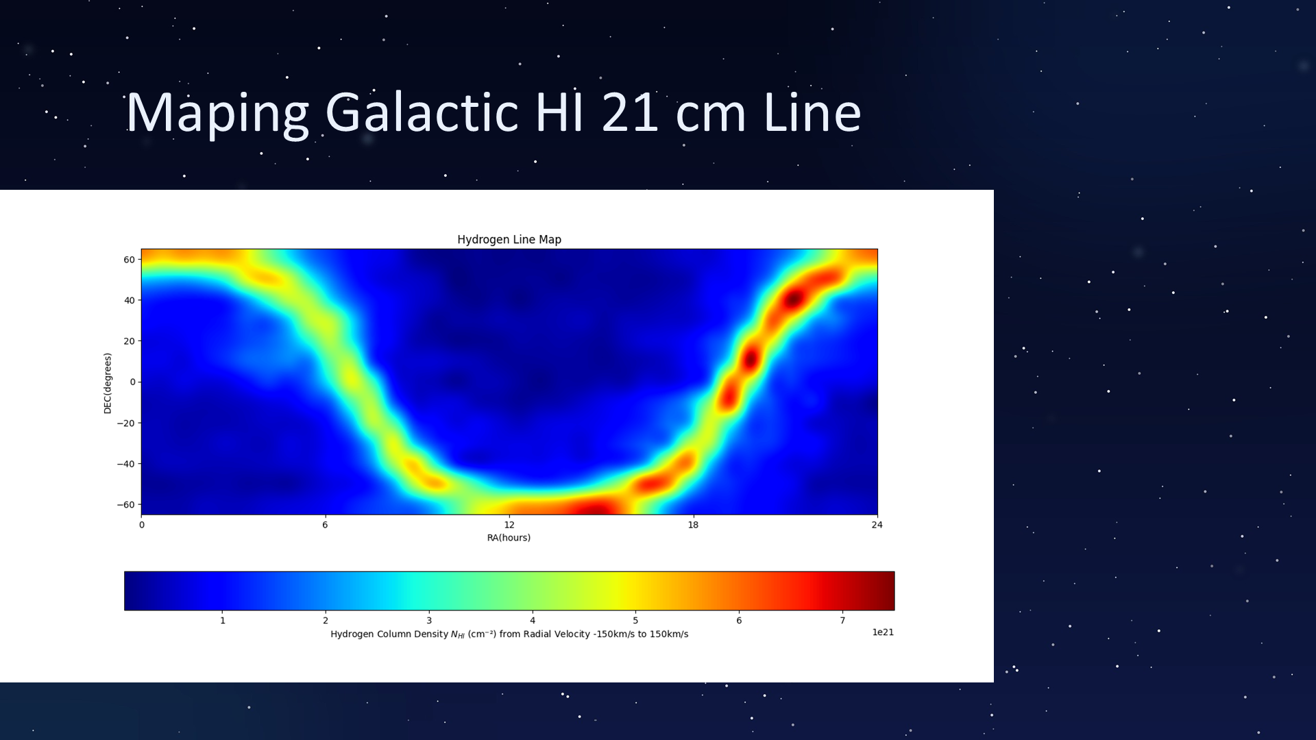
Mapping the Galactic H I 21-cm Line

Original PowerPoint slide 045: Mapping the Galactic H I 21-cm Line

Understanding this slide

This slide frames the goal as mapping the Galactic H I 21-cm line. The web title corrects the slide’s visible typo while preserving the original slide image, and the scientific idea remains the same: turn spectra into spatial information about neutral hydrogen.

Extracted slide text
  • Maping
  • Galactic HI 21 cm Line
Slide 046 / 052

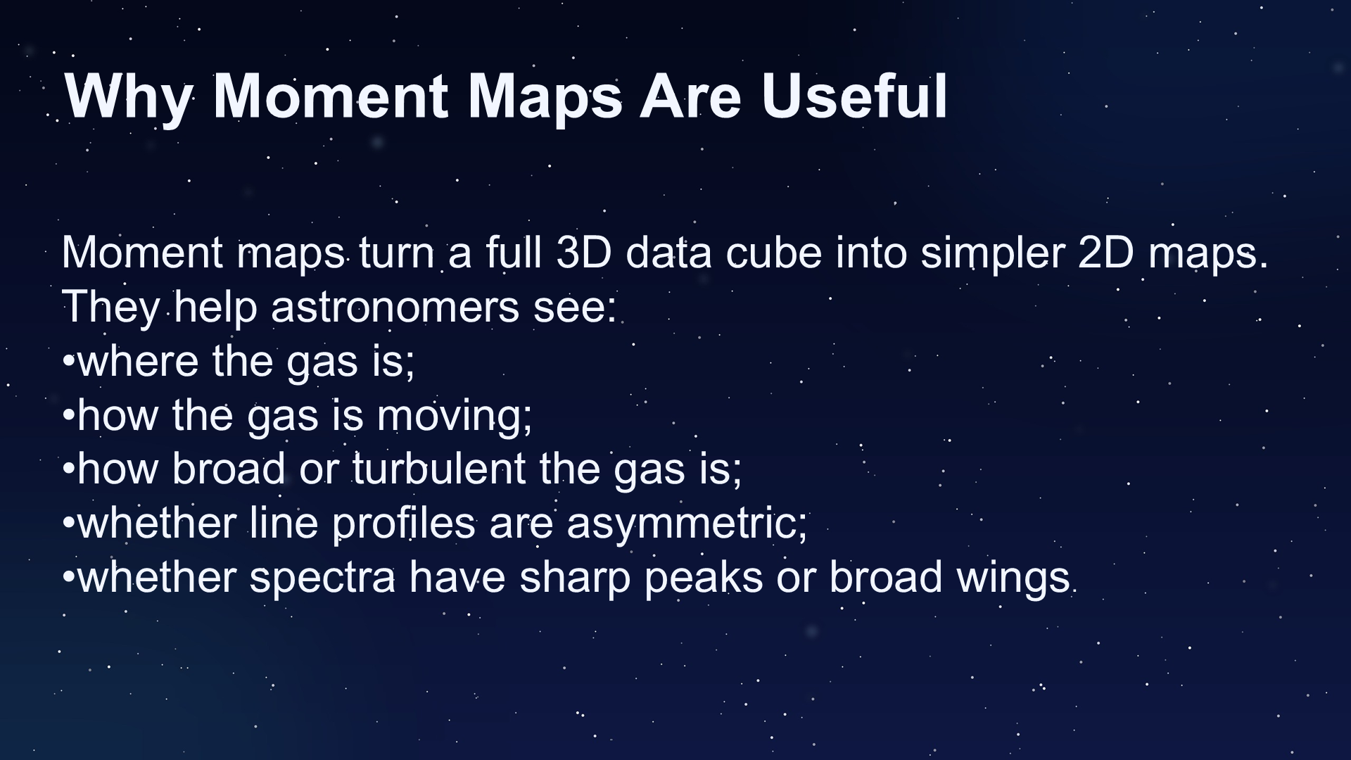
Why Moment Maps Are Useful

Original PowerPoint slide 046: Why Moment Maps Are Useful

Understanding this slide

Moment maps are useful because a full cube is rich but difficult to read all at once. They help identify where gas is located, how it is moving, and whether the line profiles are broad, asymmetric, or sharply peaked.

Extracted slide text
  • Why Moment Maps Are Useful
  • Moment maps turn a full 3D data cube into simpler 2D maps.
  • They help astronomers see:
  • where the gas is;
  • how the gas is moving;
  • how broad or turbulent the gas is;
  • whether line profiles are asymmetric;
  • whether spectra have sharp peaks or broad wings
  • .
Slide 047 / 052

What Is a Data Cube?

Original PowerPoint slide 047: What Is a Data Cube?

Understanding this slide

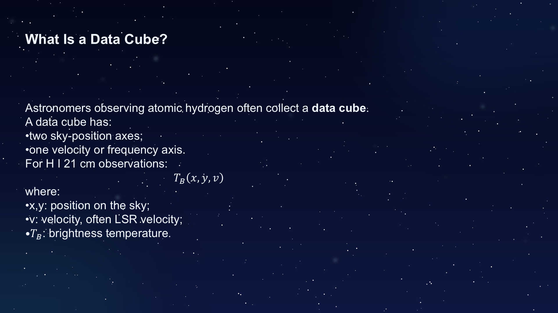
A data cube has two sky-position axes and a third frequency axis: x → sky position, y → sky position, and the third dimension → frequency. After calibration and frequency-to-velocity conversion, the same observational product becomes \(T_B(\alpha,\delta,v_{\mathrm{LSR}})\).

Extracted slide text
  • What Is a Data Cube?
  • Astronomers observing atomic hydrogen often collect a
  • data cube
  • .
  • A data cube has:
  • two sky-position axes;
  • one velocity or frequency axis.
  • For H I 21 cm observations:
  • where:
  • x,y
  • : position on the sky;
  • v: velocity, often LSR velocity;
  • ​: brightness temperature
  • .
Slide 048 / 052

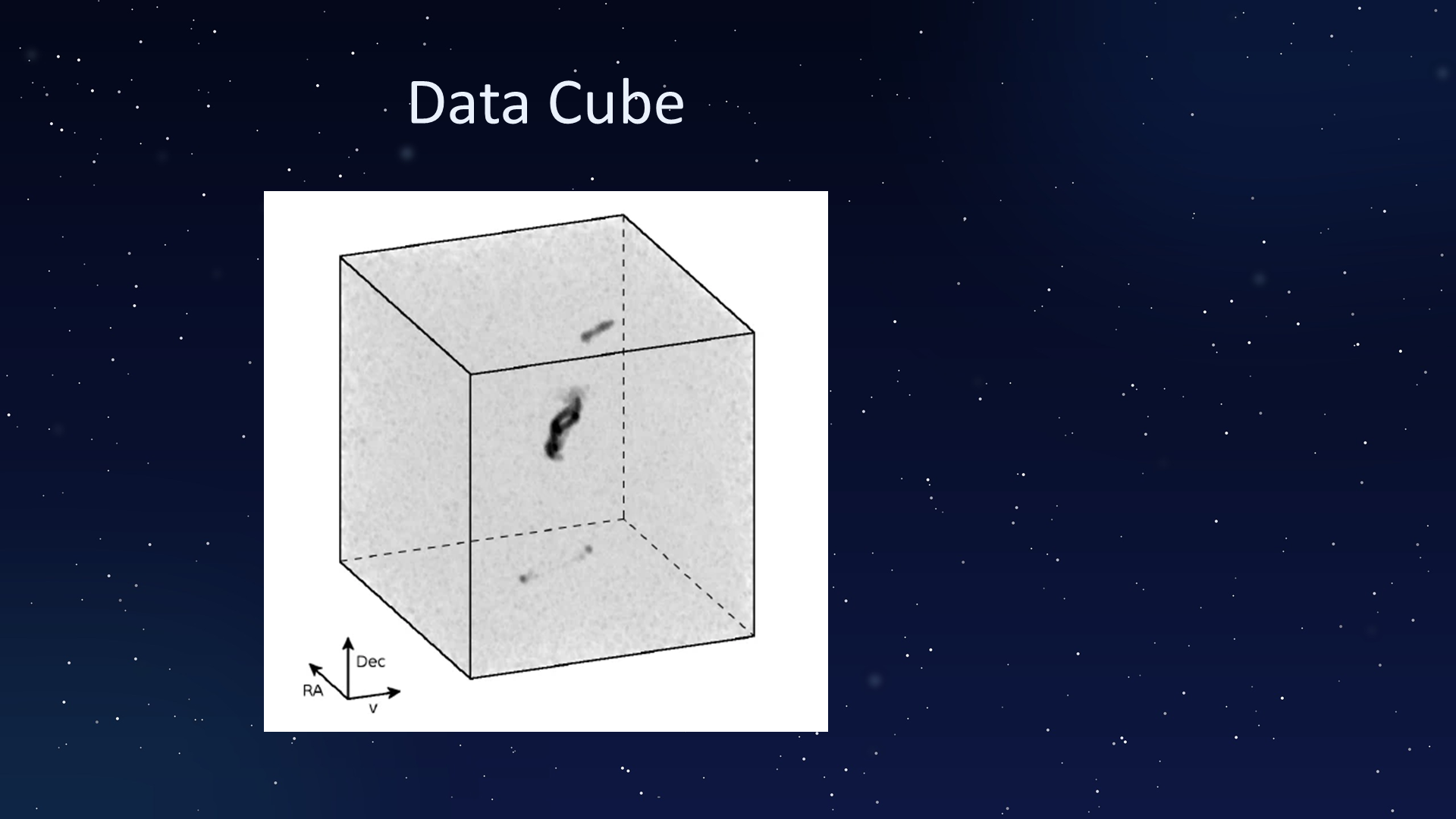
Data Cube

Original PowerPoint slide 048: Data Cube

Understanding this slide

This slide makes the cube idea visual: each sky position has a spectrum, and stacking those spectra across the observed field creates a three-dimensional object. The key is that the science is not a single image or a single spectrum, but their combination.

Extracted slide text
  • Data Cube
Slide 049 / 052

Overview of Moments

Original PowerPoint slide 049: Overview of Moments

Understanding this slide

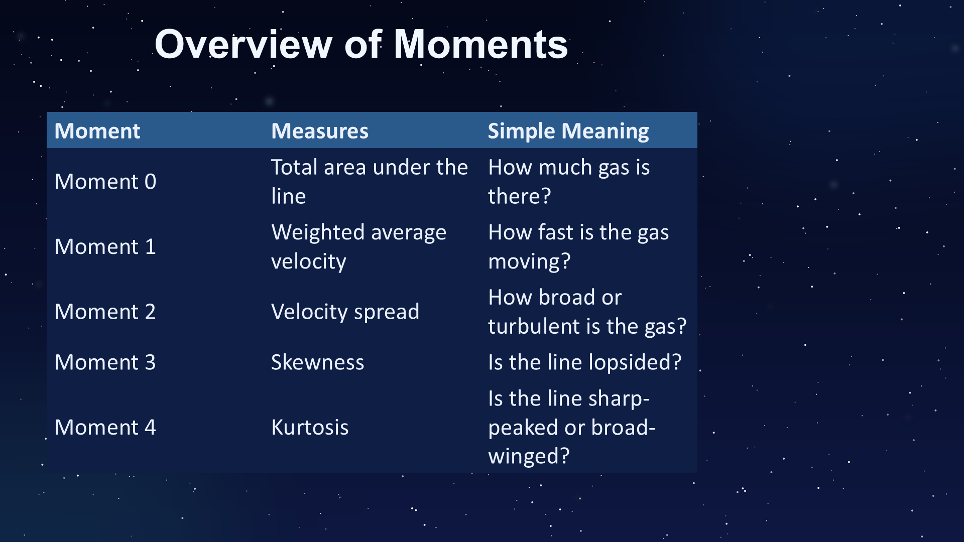
The table defines moments as summaries along the spectral dimension. Moment 0 is integrated intensity, Moment 1 is intensity-weighted mean velocity, Moment 2 is velocity dispersion, Moment 3 is skewness, and Moment 4 is kurtosis.

Extracted slide text
  • Overview of Moments
  • Moment
  • Measures
  • Simple Meaning
  • Moment 0
  • Total area under the line
  • How much gas is there?
  • Moment 1
  • Weighted average velocity
  • How fast is the gas moving?
  • Moment 2
  • Velocity spread
  • How broad or turbulent is the gas?
  • Moment 3
  • Skewness
  • Is the line lopsided?
  • Moment 4
  • Kurtosis
  • Is the line sharp-peaked or broad-winged?
Slide 050 / 052

Moments of an HI 21 cm Line Profile

Original PowerPoint slide 050: Moments of an HI 21 cm Line Profile

Understanding this slide

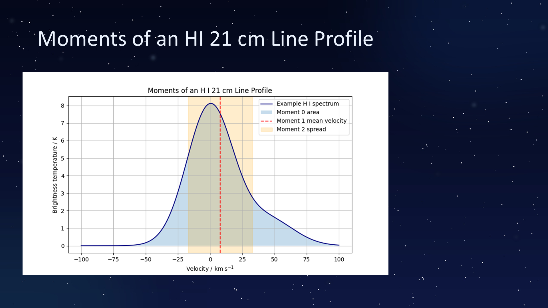
The line-profile figure shows what the moments measure on an actual spectral shape. Moments are powerful summaries, but they do not replace the original cube; they compress different aspects of the profile for interpretation.

Extracted slide text
  • Moments of an HI 21 cm Line Profile
Slide 051 / 052

H I Column Density and Galactic Mapping

Original PowerPoint slide 051: H I Column Density and Galactic Mapping

Understanding this slide

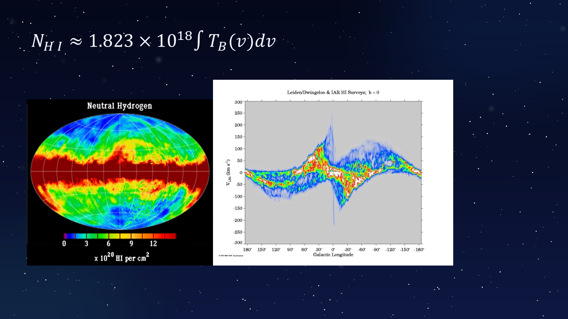
This slide connects H I brightness temperature to column density and Galactic mapping. For optically thin H I, \[N_{\mathrm{H\,I}}[\mathrm{cm^{-2}}]=1.823\times10^{18}\int T_B(v)\,dv\]; with this numerical coefficient, T_B is in kelvin and dv is conventionally in km/s. The survey imagery shows how integrating spectra across velocity becomes a map of neutral hydrogen column density.

Extracted slide text

No extractable text was found. Review the original slide image for image-only content.

Slide 052 / 052

HI 21 cm Line from KAU

Original PowerPoint slide 052: HI 21 cm Line from KAU

Understanding this slide

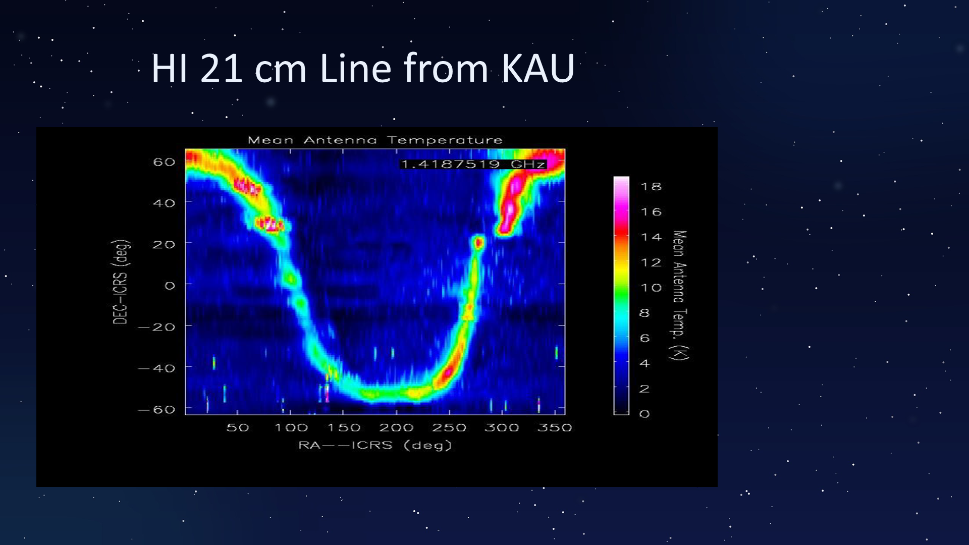
The KAU slide shows an H I 21-cm sky map at 1.4187519 GHz. The horizontal axis is RA?ICRS in degrees, the vertical axis is Dec?ICRS in degrees, and the color scale is mean antenna temperature in kelvin; the bright curved H I feature marks stronger neutral-hydrogen emission across the mapped sky positions. The slide should be read as a spatial intensity map, without inventing acquisition details that are not shown.

Extracted slide text
  • HI 21 cm Line from KAU